在深度學習的世界裡,從頭開始訓練一個模型,不只費時,還非常燒資源。更不用說為了讓訓練有效果,還得準備大量資料,這正是許多人卡關的地方。畢竟資料不是想收就收得到的。這時候一個很聰明的策略就派上用場了:如果已經有一個表現不錯的模型,能不能稍微改一下,讓它去處理我們的新任務?
當然有這個方法,而這就是所謂的遷移式學習(Transfer Learning),所以今天的內容就會帶大家從最基本的 Wx + b 開始,一步步走到如何建立一個完整的 BERT 預訓練模型。
講白一點就是把一個已經有訓練過的模型拿來做別的事,尤其是你手上的資料不多的時候特別好用。這不只可以省下一堆時間,效果通常還比你自己從頭訓練來得更穩。而像 BERT 這種模型,就是所謂的預訓練模型(Pre-trained Model)。這類型的模型在訓練時不是只學某一種任務,而是什麼都學一點、學得廣。它可以拿來做翻譯、摘要、甚至是文本生成,因為它本身在超大量的資料上訓練過,對各種語言特徵都有概念。
可以把它想像成一個很博學的人,雖然不是每一科都超強,但什麼都懂一點。你只要教它一點點新的東西,它就能舉一反三。這也是為什麼現在很多研究機構或公司會直接用這些預訓練模型,不用自己從零開始練一個,省時又省力。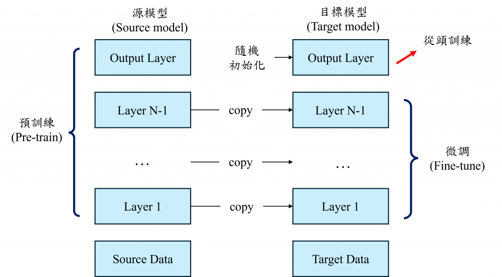
整個預訓練模型的使用流程,通常會分成預訓練跟微調(fine-tuning)兩個階段。預訓練這階段基本上都是大公司或研究機構在使用,因為他們會設計一個大型的模型架構,丟進超大量的資料裡面去訓練讓模型學會不同資料的特徵。接下來就是微調也就是我們這些一般使用者的重點,我們拿一小筆資料集,針對某個任務去調整這個預訓練模型,因為大部分的知識模型早就學好了,所以我們只需要動一些權重,讓它配合我們的任務就可以。
而在這裡模型的主體部分通常是共用權重的,而在後續的模型部分通常會不使用或不公開,而我們只需要自己加入一層分類器,讓它重新學習分類新資料,這樣效果會比較好。
不過預訓練模型的架構通常是固定好的,我們想改會有點麻煩。而且它原本訓練的資料,可能跟我們的任務不完全一樣。舉例來說如果一個模型根本沒學過怎麼做摘要,我們卻硬要拿它來做,那效果可能就不怎麼樣。所以我們在用之前,最好還是去看看它的架構是怎麼設計的、相關的論文怎麼說,這樣比較能掌握它的優缺點。
BERT(Bidirectional Encoder Representations from Transformers)是2018年由Google提出的,其模型參數設計與原始的Transformer模型並未有太多的改動,而最大的改動是它只保留了Transformer的Encoder部分與其特殊的預訓練方式,而在開始之前我們先深度理解一下BERT的模型架構
昨天我們有提到,Transformer 會用一種 Positional Encoding 的方式來處理輸入的資料,讓模型知道每個詞出現的位置,不過那個位置資訊是固定的,也就是模型本身不會去改它。但在 BERT 裡,位置的資訊是可以學習的他不只是吃進去詞語的內容,還會自己學會每個詞出現在句子中不同位置時,應該要有什麼樣的特徵。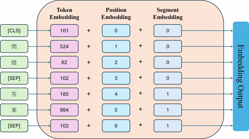
而 BERT 會用三種embedding來把句子轉換成數值資料給模型讀:
(embeddings): BertEmbeddings(
    (word_embeddings): Embedding(30522, 768, padding_idx=0)
    (position_embeddings): Embedding(512, 768)
    (token_type_embeddings): Embedding(2, 768)
    (LayerNorm): LayerNorm((768,), eps=1e-12, elementwise_affine=True)
    (dropout): Dropout(p=0.1, inplace=False)
)
如果我們要自己寫一個 BertEmbeddings 類別的話,就得依照它需要的參數大小來設定。不過在這裡我們是透過 config 的方式來設定這些參數。這麼做的好處是因為 BERT 有很多不同版本的模型,我們就可以根據所選的版本,快速載入對應的權重,不用每次都手動調整。
class BertEmbeddings(nn.Module):
    def __init__(self, config):
        super().__init__()
        self.word_embeddings = nn.Embedding(config.vocab_size, config.hidden_size, padding_idx=config.pad_token_id)
        self.position_embeddings = nn.Embedding(config.max_position_embeddings, config.hidden_size)
        self.token_type_embeddings = nn.Embedding(getattr(config, "type_vocab_size", 2), config.hidden_size)
        self.LayerNorm = nn.LayerNorm(config.hidden_size, eps=config.layer_norm_eps)
        self.dropout = nn.Dropout(config.hidden_dropout_prob)
在實作 forward 的時候,有兩點要特別留意。第一是 token_type_ids 這個參數有可能沒被傳進來,這時候我們就要預設它的值全部是 0。第二是 position_ids,這部分要根據實際輸入的長度來動態產生,例如如果輸入是 10 個字,那位置編號就會是 [0, 1, ..., 9]。這樣才能確保每個 token 都有正確的位置資訊。接下來就是整個 forward 方法的完整寫法。
def forward(self, input_ids, token_type_ids=None):
    B, T = input_ids.size()
    if token_type_ids is None:
        token_type_ids = torch.zeros_like(input_ids)

    position_ids = torch.arange(T, device=input_ids.device, dtype=torch.long).unsqueeze(0).expand(B, T)

    w = self.word_embeddings(input_ids)
    p = self.position_embeddings(position_ids)
    t = self.token_type_embeddings(token_type_ids)

    x = w + p + t
    x = self.LayerNorm(x)
    x = self.dropout(x)
    return x
我們現在看到的是 BertEncoder 的整體架構,它的核心就是一個有 12 層的 Transformer Encoder堆疊,每一層就是一個 BertLayer。乍看之下可能有點可怕,但其實可以拆解成幾個重複的小模組,而且這些模組大多就是 Transformer 裡的經典元件。
(encoder): BertEncoder(
    (layer): ModuleList(
      (0-11): 12 x BertLayer(
        (attention): BertAttention(
          (self): BertSelfAttention(
            (query): Linear(in_features=768, out_features=768, bias=True)
            (key): Linear(in_features=768, out_features=768, bias=True)
            (value): Linear(in_features=768, out_features=768, bias=True)
            (dropout): Dropout(p=0.1, inplace=False)
          )
          (output): BertSelfOutput(
            (dense): Linear(in_features=768, out_features=768, bias=True)
            (dropout): Dropout(p=0.1, inplace=False)
            (LayerNorm): LayerNorm((768,), eps=1e-12, elementwise_affine=True)
          )
        )
        (intermediate): BertIntermediate(
          (dense): Linear(in_features=768, out_features=3072, bias=True)
          (intermediate_act_fn): GELU(approximate='none')
        )
        (output): BertOutput(
          (dense): Linear(in_features=3072, out_features=768, bias=True)
          (dropout): Dropout(p=0.1, inplace=False)
          (LayerNorm): LayerNorm((768,), eps=1e-12, elementwise_affine=True)
        )
      )
    )
  )
這個模組負責看哪裡重要,也就是我們常說的 Attention 機制。它裡面有三個 Linear layer,分別做出 Query, Key, Value,這跟我們昨天提到的 Self-Attention 概念完全一樣。
它會把這三個東西 reshape 成Multi-head Attention 需要的格式。接著就是計算 Attention Score,並經過 Softmax,再加上一點 Dropout處理Attention Weight,最後會把算出來的Attention Weight跟 Value 做乘法,得到我們的Attention結果。
class BertSelfAttention(nn.Module):
    def __init__(self, config):
        super().__init__()
        if config.hidden_size % config.num_attention_heads != 0:
            raise ValueError("hidden_size must be divisible by num_attention_heads")
        self.num_attention_heads = config.num_attention_heads
        self.attention_head_size = config.hidden_size // config.num_attention_heads
        self.all_head_size = self.num_attention_heads * self.attention_head_size

        self.query = nn.Linear(config.hidden_size, self.all_head_size)
        self.key = nn.Linear(config.hidden_size, self.all_head_size)
        self.value = nn.Linear(config.hidden_size, self.all_head_size)

        self.dropout = nn.Dropout(config.attention_probs_dropout_prob)

    def transpose_for_scores(self, x):
        new_shape = x.size()[:-1] + (self.num_attention_heads, self.attention_head_size)
        x = x.view(*new_shape)  # [B, T, nh, hd]
        return x.permute(0, 2, 1, 3)  # [B, nh, T, hd]

    def forward(self, hidden_states, attention_mask=None):
        q = self.query(hidden_states)
        k = self.key(hidden_states)
        v = self.value(hidden_states)

        q = self.transpose_for_scores(q)
        k = self.transpose_for_scores(k)
        v = self.transpose_for_scores(v)

        attn_scores = torch.matmul(q, k.transpose(-1, -2)) / math.sqrt(self.attention_head_size)  # [B, nh, T, T]
        if attention_mask is not None:
            attn_scores = attn_scores + attention_mask

        attn_probs = F.softmax(attn_scores, dim=-1)
        attn_probs = self.dropout(attn_probs)

        context = torch.matmul(attn_probs, v)  # [B, nh, T, hd]
        context = context.permute(0, 2, 1, 3).contiguous()
        new_context_shape = context.size()[:2] + (self.all_head_size,)
        context = context.view(*new_context_shape)  # [B, T, H]
        return context
其實在 BertSelfOutput 裡,有個很關鍵的步驟,就是 Transformer 裡常見的 Add & Norm。簡單來說,它就是先把 Attention 的輸出再經過一層 Linear,然後加上 Dropout,接著再把這個結果跟原本進來的輸入做個 skip connection,最後再做 Layer Normalization。這樣做的目的是為了讓訓練過程更穩定。
class BertSelfOutput(nn.Module):
    def __init__(self, config):
        super().__init__()
        # name: attention.output.dense
        self.dense = nn.Linear(config.hidden_size, config.hidden_size)
        self.dropout = nn.Dropout(config.hidden_dropout_prob)
        # name: attention.output.LayerNorm
        self.LayerNorm = nn.LayerNorm(config.hidden_size, eps=config.layer_norm_eps)

    def forward(self, hidden_states, input_tensor):
        hidden_states = self.dense(hidden_states)
        hidden_states = self.dropout(hidden_states)
        hidden_states = self.LayerNorm(hidden_states + input_tensor) # Skip Connection
        return hidden_states
每層 Transformer 結尾的一個重要部分,主要是用來進一步轉換和處理前面得到的資訊。它被拆成兩個部分來進行,首先是 BertIntermediate,這裡會先用一層 Linear 把原本的 768 維向量放大成 3072 維,接著通過一個GELU來處理它的線性變換(這裡也是唯一跟Transformer不同的地方)。
class BertIntermediate(nn.Module):
    def __init__(self, config):
        super().__init__()
        # name: intermediate.dense
        self.dense = nn.Linear(config.hidden_size, config.intermediate_size)
        self.intermediate_act_fn = nn.GELU()

    def forward(self, hidden_states):
        return self.intermediate_act_fn(self.dense(hidden_states))
然後是 BertOutput,它再把剛剛拉高的 3072 維壓回到原來的 768 維。最後跟之前 Attention Output 的流程很像先做 Dropout,再加上原始輸入的 Skip Connection,然後做 Layer Normalization,這整個流程有助於模型更穩定地學習。
class BertOutput(nn.Module):
    def __init__(self, config):
        super().__init__()
        # name: output.dense
        self.dense = nn.Linear(config.intermediate_size, config.hidden_size)
        self.dropout = nn.Dropout(config.hidden_dropout_prob)
        # name: output.LayerNorm
        self.LayerNorm = nn.LayerNorm(config.hidden_size, eps=config.layer_norm_eps)

    def forward(self, hidden_states, input_tensor):
        hidden_states = self.dense(hidden_states)
        hidden_states = self.dropout(hidden_states)
        hidden_states = self.LayerNorm(hidden_states + input_tensor) # Skip Connection
        return hidden_states
你會發現整個 BERT Encoder 的定義基本上與我們的Transformer根本沒有差異,而現在我們只需要建立BertLayer與BertEncoder就能完成整個模型的建立了,而這樣的設計只是為了方便動態調動多層Transformer
class BertLayer(nn.Module):
    def __init__(self, config):
        super().__init__()
        self.attention = BertAttention(config)
        self.intermediate = BertIntermediate(config)
        self.output = BertOutput(config)

    def forward(self, hidden_states, attention_mask=None):
        attention_output = self.attention(hidden_states, attention_mask)
        intermediate_output = self.intermediate(attention_output)
        layer_output = self.output(intermediate_output, attention_output)
        return layer_output
而我們經過前面的建立現在就能夠只使用簡單幾行就完成 Transformer Layer 的精髓了,雖然你在這邊沒看到像昨天的明顯加法或 LayerNorm,這是因為再HF架構中的BERT把skip connection 都藏在 Attention 跟 Output 裡面(我上面程式碼註解的地方)。
而BertEncoder則是進行實際堆疊的地方,不過在HF風格上通常會有一個 output_hidden_states=True,它也會幫你把每一層的輸出都存下來,這對於分析模型或做視覺化非常有用。
class BertEncoder(nn.Module):
    def __init__(self, config):
        super().__init__()
        # name path: encoder.layer.0 ... encoder.layer.N
        self.layer = nn.ModuleList([BertLayer(config) for _ in range(config.num_hidden_layers)])

    def forward(self, hidden_states, attention_mask=None, output_hidden_states=False):
        all_hidden_states = [] if output_hidden_states else None
        for layer_module in self.layer:
            if output_hidden_states:
                all_hidden_states.append(hidden_states)
            hidden_states = layer_module(hidden_states, attention_mask)
        if output_hidden_states:
            all_hidden_states.append(hidden_states)
        return hidden_states, all_hidden_states
BERT Encoder 看起來很複雜,但其實就是 12 層完全一樣的 Transformer 結構堆起來。每層做注意力 → 前饋網路 → skip,加起來就可以學到上下文關係。
當我們把一句話丟進 BERT 模型裡,它其實不會馬上就開始「理解」文字,而是會先幫句子加上一些特別的符號,例如 [CLS] 和 [SEP],簡單來說:
單一句子: [CLS] 句子 [SEP]
兩句話:   [CLS] 句子A [SEP] 句子B [SEP]
而[SEP] 是用來分隔句子的,像是句子中間的逗號,也順便當作句尾。那開頭的 [CLS] 呢?這就比較特別了。雖然一開始它只是個空白 token,沒什麼意思,但 BERT 會訓練它變成整句話的代表,就像是一個總結整句意思的代言人。
為什麼它可以代表整句話?這就要靠 Transformer 裡厲害的東西Self-Attention 機制。它的概念有點像是每個詞都會去注意整句話裡其他詞,看看彼此的關聯性。就算詞在句首或句尾,都會把整句的資訊融合進來,只是每個詞吸收的重點可能不同。
數學上在做什麼?其實就是幫每個詞算出對 [CLS] 來說,它有多重要,也就是softmax((Q · K.T) / sqrt(d)),而些注意力分數會用來加權每個詞的 Value(V),再全部加總起來,因此CLS 就像是一個訊息總管,根據自己的關注程度去吸收其他詞的資訊,最後變成它的新向量。
因此到這時候就輪到 BertPooler 出場了雖然模型裡寫得很簡單:
(pooler): BertPooler(
    (dense): Linear(in_features=768, out_features=768, bias=True)
    (activation): Tanh()
)
但重點是它只拿 [CLS] 的向量來用,也就是在程式裡會看到hidden_states[:, 0]意思就是只抓第一個 token,也就是 [CLS] 的位置。這個 [CLS] 的向量會先丟進一個 Linear 層做轉換,再經過一個 Tanh 函數做激活,讓輸出的值被限制在 -1 到 1 之間,讓後面的模型更好的進行分類或運算。
class BertPooler(nn.Module):
    def __init__(self, config):
        super().__init__()
        self.dense = nn.Linear(config.hidden_size, config.hidden_size)
        self.activation = nn.Tanh()

    def forward(self, hidden_states):
        first_token_tensor = hidden_states[:, 0]
        pooled_output = self.dense(first_token_tensor)
        pooled_output = self.activation(pooled_output)
        return pooled_output
講到這邊,其實我們已經把 BERT 的整體模型架構講得差不多了。不過要注意這還不是全部!我們現在談的主要是 模型的底層架構,也就是 BERT 怎麼處理文字、怎麼用 Self-Attention、怎麼透過 [CLS] 來代表整句話,但實際上,BERT 在做預訓練時,還會在這個基礎上加上一些額外的分類器。
這些分類器有點像是訓練小助手,專門幫助模型學會更準確地用 [CLS] 去做各種任務,而使用這些訓練技巧,會讓 [CLS] 的表示學得更有意義,也就是我們俗稱的「讓它更懂句子」。不過這部分就留到明天再說吧,今天先消化一下這些架構和機制,不然一次塞太多,頭腦真的會轉不過來。
今天我們介紹了 https://huggingface.co/google-bert/bert-base-uncased 這個模型架構,順便用程式碼來幫助你更清楚理解 BERT 的原理。這個架構其實你也可以直接套用我貼的連結裡的預訓練權重,不過這部分我們會留到後面再詳細說明。
明天我們會進一步聊聊BERT 是怎麼被訓練出來的?它到底學了哪些東西? 還有在訓練過程中加入的一些小技巧,像是 MLM(Masked Language Modeling)和 NSP(Next Sentence Prediction),這些又是怎麼幫助 BERT 更懂語言的?


 iThome鐵人賽