Loading & exploring house sale data

今天要來實作一個跟回歸分析相關的題目，我們將引用課程提供的房價訊息(King County data)，其位於美國西雅圖

我們將用這個資料來做回歸預測房價

首先我們必須先引入 Graph Lab

import graphlab

接著導入房價的資料(home_data.gl)，我們也可以透過graphlab來讓資料視覺化

seles = graphlab.SFrame('/home/user/nylon7/machine_learning/week1/home_data.gl/')
seles
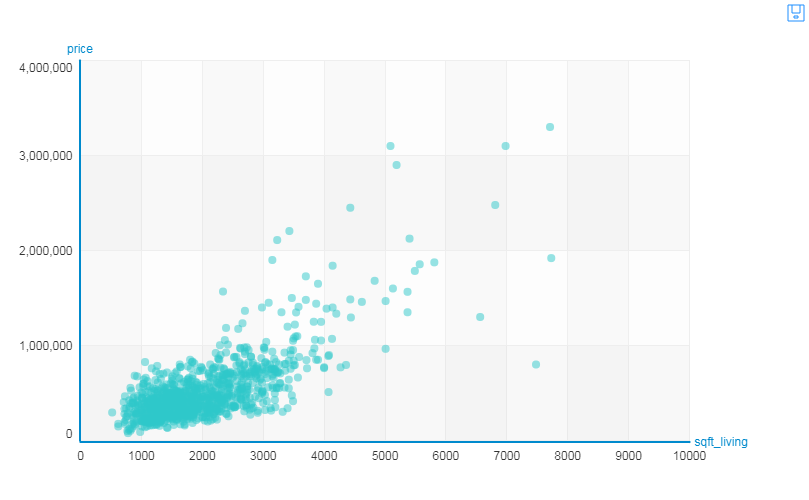
seles.show(view="Scatter Plot",x="sqft_living",y="price")

我們可以發現，這張圖大部分的情況都符合我們直覺的反應，房子地坪越大，價格越高

Splitting the data into training and test sets

接著我們想要建立一個回歸的模型，所以最重要的是，我們要先處理測試集與訓練集

所以我們必須把資料分成測試集與訓練集

我們呼叫隨機分布函數(random_split())

#.8 意味著 80%訓練集/20%測試集
train_data,test_data = seles.random_split(.8,seed=0)

Learning a simple regression model to predict house prices from house size

有了測試集與訓練集之後，接下來就是建立回歸模型(在這次的課程當中只會先用內建的演算法)

# 預測目標為"價格"，特徵為"房子大小"
sqft_model = graphlab.linear_regression.create(train_data,target='price',features=['sqft_living'])

我們將得到一個圖表，它使用的演算法為Newton's method(graphlab 除非指定否則會自動選擇)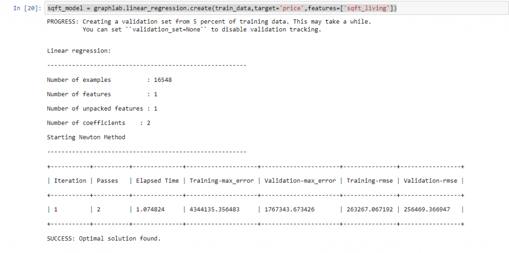

Evaluating error (RMSE) of the simple model

我們可以從測試集裡面取得平均的價格

接著可以從之前建立的模型呼叫它的評估函數，它會返回一些資料告訴我們擬合的狀況

print test_data['price'].mean()
#543,000
print sqft_model.evaluate(test_data)
#{'max_error': 4130610.392309714, 'rmse': 255224.89364924902}

此例的西雅圖均價為543,000

測試資料的最大誤差為410萬，我們可以從中推敲一定有一個房子的資料是異常，導致這個模型預測的不夠精確

RMSE(方均根差)是種在測量數值之間差異的量度

Visualizing predictions of simple model with Matplotlib

接下來我們要顯示我們的預測

import matplotlib.pyplot as plt

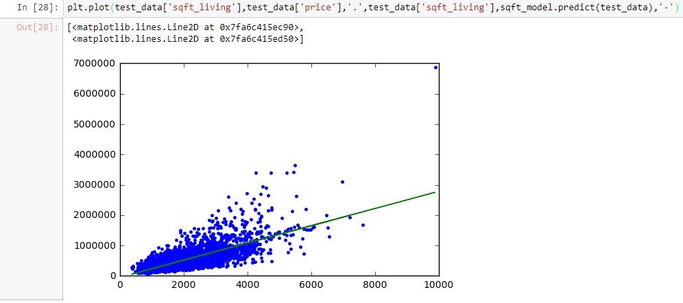
#用test_data作為參數，房子大小為X軸價格為Y軸，並以dot表示每一個測試
#接著是預測的線，房子大小依然為X軸，Y軸則為預測價格，並以'-'來繪製
plt.plot(test_data['sqft_living'],test_data['price'],'.',
         test_data['sqft_living'],sqft_model.predict(test_data),'-')

後記

還有一半還沒完成，今天錯估了形勢，以為已經安裝成功，結果沒想到爆出這種錯誤，還好有線上的jupyter可用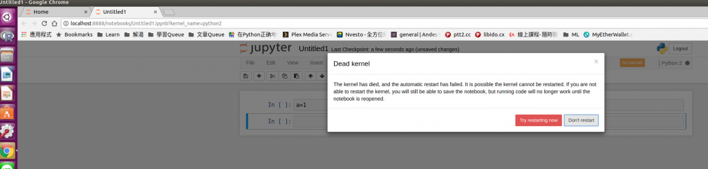

不只如此，用makedown畫那張房價資料圖，讓我差點崩潰QQ

Reference:

• Machine Learning Foundations: A Case Study Approach 華盛頓大學在 coursera 上的公開課程，為本筆記追蹤的主要素材