Decision Tree 決策樹,因為它可以用很多決策點排列的像聖誕樹依樣。如果要分類三種主題相片:火山、海洋、森林,可能可以依照下圖樹枝狀排列,火山可能有岩漿紅色偏多(R>200)、海洋藍色偏多(B>100)、剩下的圖片只要有綠色可能就有森林(G>30)。這些特徵都可以作為一個節點,節點的順序先後會有不同結果。要分幾個節點哪個要擺第一?就需要了解一下決策樹演算法~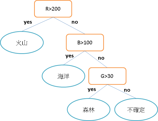
如下圖我們想從30位學生中找出有打板球15位學生,左圖用性別做區分右圖用班級做區分。很合理的猜測男生一定是比較喜歡運動用性別應該有不錯效果,而用班級區分除非有體育班否則兩分類結果應該雷同。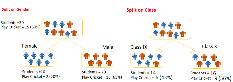
數學上常用 Information Gain 及 Gini Index 來定義分的好壞程度:
翻譯成資訊獲利,類似是熵Entropy。念物理系應該蠻好理解的大三的熱力學,也可以說是比較亂度!
Entropy = -p * log2 p – q * log2q
p:成功的機率(或true的機率) q:失敗的機率(或false的機率)
當所有的資料都是相同一致,它們的Entropy就是0,如果資料各有一半不同,那麼Entropy就是1
1.來計算一下母節點的熵為 -(15/30) log2 (15/30) – (15/30) log2 (15/30) = 1 需要分類
2.用性別做節點 -(2/10) log2 (2/10) – (8/10) log2 (8/10) = 0.72
-(13/20) log2 (13/20) – (7/20) log2 (7/20) = 0.93
加權後為:(10/30)*0.72 + (20/30)*0.93 = 0.86
3.用班級做節點 -(6/14) log2 (6/14) – (8/14) log2 (8/14) = 0.99
-(9/16) log2 (9/16) – (7/16) log2 (7/16) = 0.99
加權後為:(14/30)*0.99 + (16/30)*0.99 = 0.99
0.99 > 0.86 因此系統會先選擇用性別做節點,先從熵最小的開始
Gini係數公式為p2+q2
1.用性別分類
Femail節點:十位女性,其中有2位打板球10位不打,Gini係數為
(0.2)2+(0.8)2=0.68
Male節點:20位男性,其中有13位打板球7位不打,Gini係數為
(0.65)2+(0.35)2=0.55
因此以性別分類的Gini係數加權後為:(10/30)*0.68+(20/30)*0.55 = 0.59。
2.用班級分類
Class IX節點:此班14位同學,其中6位打板球8位不打,因此Gini係數為
(0.43)2+(0.57)2=0.51
Class X節點:此班16位同學,其中9位打板球7位不打,因此Gini係數為
(0.56)2+(0.44)2=0.51
因此以班級分類的決策樹,其Gini係數加權結果:(14/30)*0.51+(16/30)*0.51 = 0.51。兩樹相互比較,以性別分類的吉尼係數大於以班級分類,因此系統會採用性別來進行節點的分類。
決策樹很容易產生Overfitting如果不限制它,它可以一直長下去分得過細。所以有以下常用的幾種方法來設限:
設限
Minimum samples for a node split:資料數目不得小於多少才能再產生新節點。
Minimum samples for a terminal node (leaf):要成為葉節點,最少需要多少資料。
Maximum depth of tree (vertical depth):限制樹的高度最多幾層。
Maximum number of terminal nodes:限制最終葉節點的數目
Maximum features to consider for split:在分離節點時,最多考慮幾種特徵值。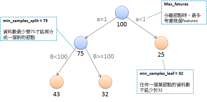
現在來照著步驟使用iris資料集做一次決策樹分類
%matplotlib inline
from sklearn import datasets
import pandas as pd
import numpy as np
import matplotlib.pyplot as plt
import seaborn as sns
iris = datasets.load_iris()
x = pd.DataFrame(iris['data'], columns=iris['feature_names'])
print("target_names: "+str(iris['target_names']))
y = pd.DataFrame(iris['target'], columns=['target'])
iris_data = pd.concat([x,y], axis=1)
iris_data = iris_data[['sepal length (cm)','petal length (cm)','target']]
iris_data = iris_data[iris_data['target'].isin([0,1])]
iris_data.head(3)
from sklearn.model_selection import train_test_split
X_train, X_test, y_train, y_test = train_test_split(
    iris_data[['sepal length (cm)','petal length (cm)']], iris_data[['target']],
    test_size=0.3, random_state=0)
from sklearn.tree import DecisionTreeClassifier
tree = DecisionTreeClassifier(criterion = 'entropy', random_state=0)
iris_data['target_class'] = iris_data['target_name'].map(target_class)
tree.fit(X_train,y_train)
y_test['target'].values
error = 0
for i, v in enumerate(tree.predict(X_test)):
    if v!= y_test['target'].values[i]:
        print(i,v)
        error+=1
print(error)
tree.score(X_test,y_test['target'])
from matplotlib.colors import ListedColormap

def plot_decision_regions(X, y, classifier, test_idx=None, resolution=0.02):

    # setup marker generator and color map
    markers = ('s', 'x', 'o', '^', 'v')
    colors = ('red', 'blue', 'lightgreen', 'gray', 'cyan')
    cmap = ListedColormap(colors[:len(np.unique(y))])

    # plot the decision surface
    x1_min, x1_max = X[:, 0].min() - 1, X[:, 0].max() + 1
    x2_min, x2_max = X[:, 1].min() - 1, X[:, 1].max() + 1
    xx1, xx2 = np.meshgrid(np.arange(x1_min, x1_max, resolution),
                           np.arange(x2_min, x2_max, resolution))
    Z = classifier.predict(np.array([xx1.ravel(), xx2.ravel()]).T)
    Z = Z.reshape(xx1.shape)
    plt.contourf(xx1, xx2, Z, alpha=0.4, cmap=cmap)
    plt.xlim(xx1.min(), xx1.max())
    plt.ylim(xx2.min(), xx2.max())

    for idx, cl in enumerate(np.unique(y)):
        plt.scatter(x=X[y == cl, 0],
                    y=X[y == cl, 1],
                    alpha=0.6,
                    c=cmap(idx),
                    edgecolor='black',
                    marker=markers[idx],
                    label=cl)

    # highlight test samples
    if test_idx:
        # plot all samples
        if not versiontuple(np.__version__) >= versiontuple('1.9.0'):
            X_test, y_test = X[list(test_idx), :], y[list(test_idx)]
            warnings.warn('Please update to NumPy 1.9.0 or newer')
        else:
            X_test, y_test = X[test_idx, :], y[test_idx]

        plt.scatter(X_test[:, 0],
                    X_test[:, 1],
                    c='',
                    alpha=1.0,
                    edgecolor='black',
                    linewidths=1,
                    marker='o',
                    s=55, label='test set')
plot_decision_regions(X_train.values, y_train['target'].values, classifier=tree)
plt.xlabel('petal length [standardized]')
plt.ylabel('petal width [standardized]')
plt.legend(loc='upper left')
plt.tight_layout()
plt.show()
from sklearn.tree import export_graphviz
iris = datasets.load_iris()
x = pd.DataFrame(iris['data'], columns=iris['feature_names'])
print("target_names: "+str(iris['target_names']))
y = pd.DataFrame(iris['target'], columns=['target'])
iris_data = pd.concat([x,y], axis=1)
iris_data = iris_data[['petal width (cm)','petal length (cm)','target']]
iris_data.head(3)
X_train, X_test, y_train, y_test = train_test_split(
    iris_data[['petal width (cm)','petal length (cm)']], iris_data[['target']], test_size=0.3, random_state=0)

from sklearn.tree import DecisionTreeClassifier
tree = DecisionTreeClassifier(criterion = 'entropy', max_depth=3, random_state=0)
tree.fit(X_train,y_train)
plot_decision_regions(X_train.values, y_train['target'].values, classifier=tree)
plt.xlabel('petal length [standardized]')
plt.ylabel('petal width [standardized]')
plt.legend(loc='upper left')
plt.tight_layout()
plt.show()
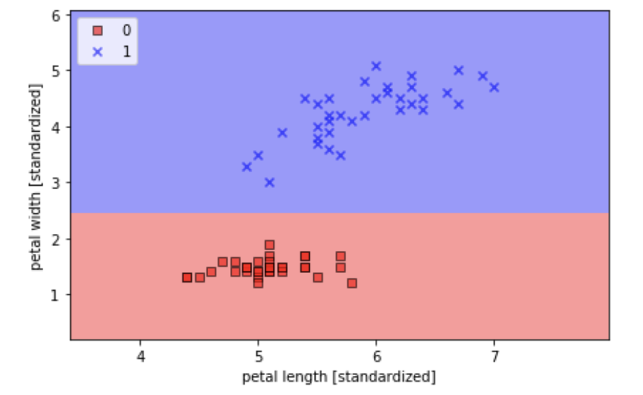
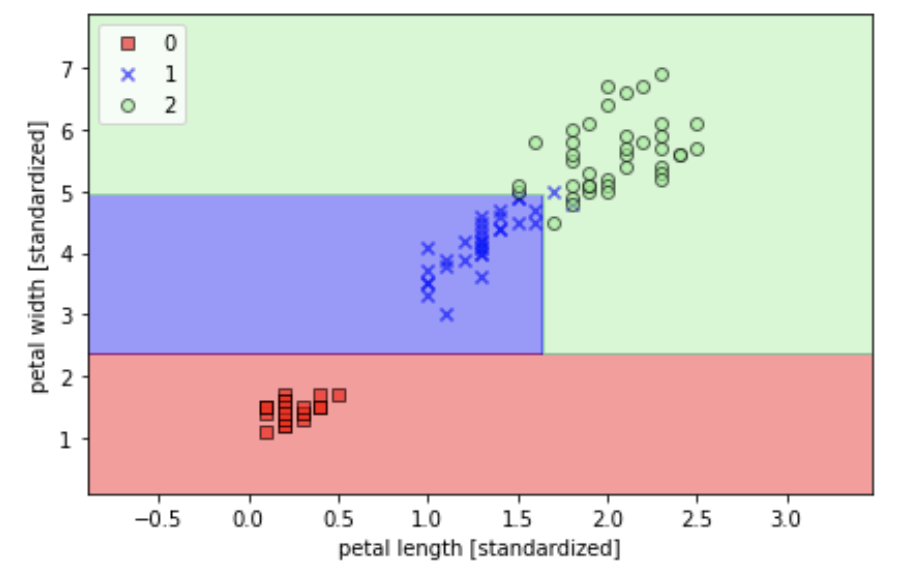
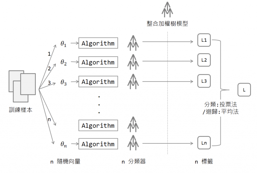
上圖分別是分兩類與三類的結果真的切蠻細的,關於Random Forest的原理大致上是多個決策樹一起做決定也消耗較多計算能力。詳細流程蠻複雜的這裡就不多作介紹XD有興趣可從參考網站了解一下