參考網站

昨天的感知器只能分類不能知道機率是多少，但Logistic regression可以求得機率！既然有機率也就是可以拿來算賠率的意思＠＠

邏輯斯回歸 Logistic regression

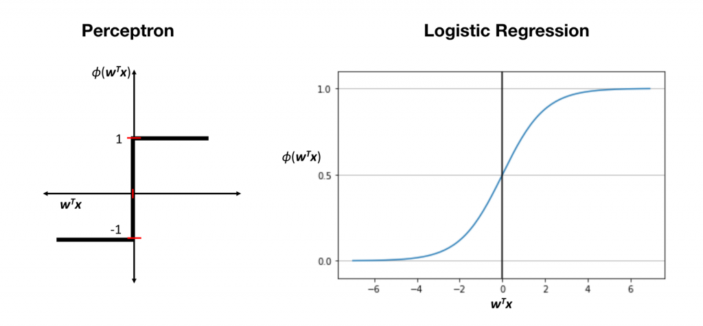
首先它並不是一個回歸模型！來看一下他跟感知器的差別～其實就是差在多了Logistic函數，它是個平滑曲線 z > 0 時機率大於 0.5(+1類)，z < 0時機率小於 0.5(-1類)。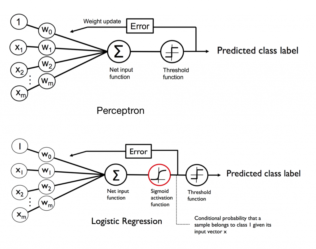


Logistic 函數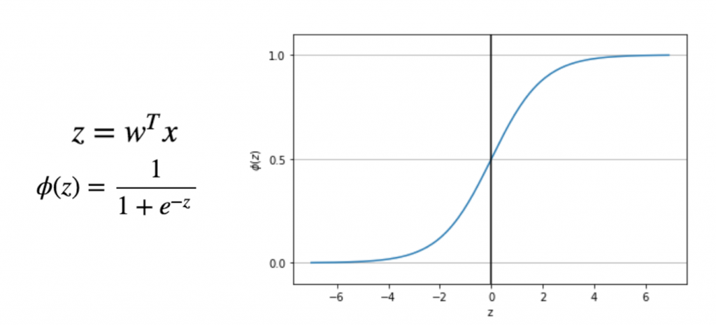

接下來照著步驟使用iris資料集試跑一下

from sklearn import datasets
import pandas as pd
import numpy as np
import matplotlib.pyplot as plt
import seaborn as sns
%matplotlib inline
iris = datasets.load_iris()
x = pd.DataFrame(iris['data'], columns=iris['feature_names'])
print("target_names: "+str(iris['target_names']))
y = pd.DataFrame(iris['target'], columns=['target'])
iris_data = pd.concat([x,y], axis=1)
iris_data = iris_data[['sepal length (cm)','petal length (cm)','target']]
iris_data = iris_data[iris_data['target'].isin([0,1])]
iris_data.head(3)
from sklearn.model_selection import train_test_split
X_train, X_test, y_train, y_test = train_test_split(
    iris_data[['sepal length (cm)','petal length (cm)']], iris_data[['target']], test_size=0.3, random_state=0)
len(X_train)
X_test
len(X_test)
from sklearn.preprocessing import StandardScaler

sc = StandardScaler()
sc.fit(X_train)
X_train_std = sc.transform(X_train)
X_test_std = sc.transform(X_test)
X_train_std
from IPython.display import Math
Math(r'z=w^Tx')
Math(r'\phi{(z)}=\frac{1}{1+e^{-z}}')
import matplotlib.pyplot as plt
import numpy as np


def sigmoid(z):
    return 1.0 / (1.0 + np.exp(-z))

z = np.arange(-7, 7, 0.1)
phi_z = sigmoid(z)

plt.plot(z, phi_z)
plt.axvline(0.0, color='k')
plt.ylim(-0.1, 1.1)
plt.xlabel('z')
plt.ylabel('$\phi (z)$')

# y axis ticks and gridline
plt.yticks([0.0, 0.5, 1.0])
ax = plt.gca()
ax.yaxis.grid(True)

plt.tight_layout()
# plt.savefig('./figures/sigmoid.png', dpi=300)
plt.show()
y_train['target'].values
from sklearn.linear_model import LogisticRegression
lr = LogisticRegression()
lr.fit(X_train_std,y_train['target'].values)
from matplotlib.colors import ListedColormap

def plot_decision_regions(X, y, classifier, test_idx=None, resolution=0.02):

    # setup marker generator and color map
    markers = ('s', 'x', 'o', '^', 'v')
    colors = ('red', 'blue', 'lightgreen', 'gray', 'cyan')
    cmap = ListedColormap(colors[:len(np.unique(y))])

    # plot the decision surface
    x1_min, x1_max = X[:, 0].min() - 1, X[:, 0].max() + 1
    x2_min, x2_max = X[:, 1].min() - 1, X[:, 1].max() + 1
    xx1, xx2 = np.meshgrid(np.arange(x1_min, x1_max, resolution),
                           np.arange(x2_min, x2_max, resolution))
    Z = classifier.predict(np.array([xx1.ravel(), xx2.ravel()]).T)
    Z = Z.reshape(xx1.shape)
    plt.contourf(xx1, xx2, Z, alpha=0.4, cmap=cmap)
    plt.xlim(xx1.min(), xx1.max())
    plt.ylim(xx2.min(), xx2.max())

    for idx, cl in enumerate(np.unique(y)):
        plt.scatter(x=X[y == cl, 0], 
                    y=X[y == cl, 1],
                    alpha=0.6, 
                    c=cmap(idx),
                    edgecolor='black',
                    marker=markers[idx], 
                    label=cl)

    # highlight test samples
    if test_idx:
        # plot all samples
        if not versiontuple(np.__version__) >= versiontuple('1.9.0'):
            X_test, y_test = X[list(test_idx), :], y[list(test_idx)]
            warnings.warn('Please update to NumPy 1.9.0 or newer')
        else:
            X_test, y_test = X[test_idx, :], y[test_idx]

        plt.scatter(X_test[:, 0],
                    X_test[:, 1],
                    c='',
                    alpha=1.0,
                    edgecolor='black',
                    linewidths=1,
                    marker='o',
                    s=55, label='test set')
plot_decision_regions(X_train_std, y_train['target'].values, classifier=lr)
plt.xlabel('sepal length (cm) [standardized]')
plt.ylabel('petal width [standardized]')
plt.legend(loc='upper left')
plt.tight_layout()
plt.show()

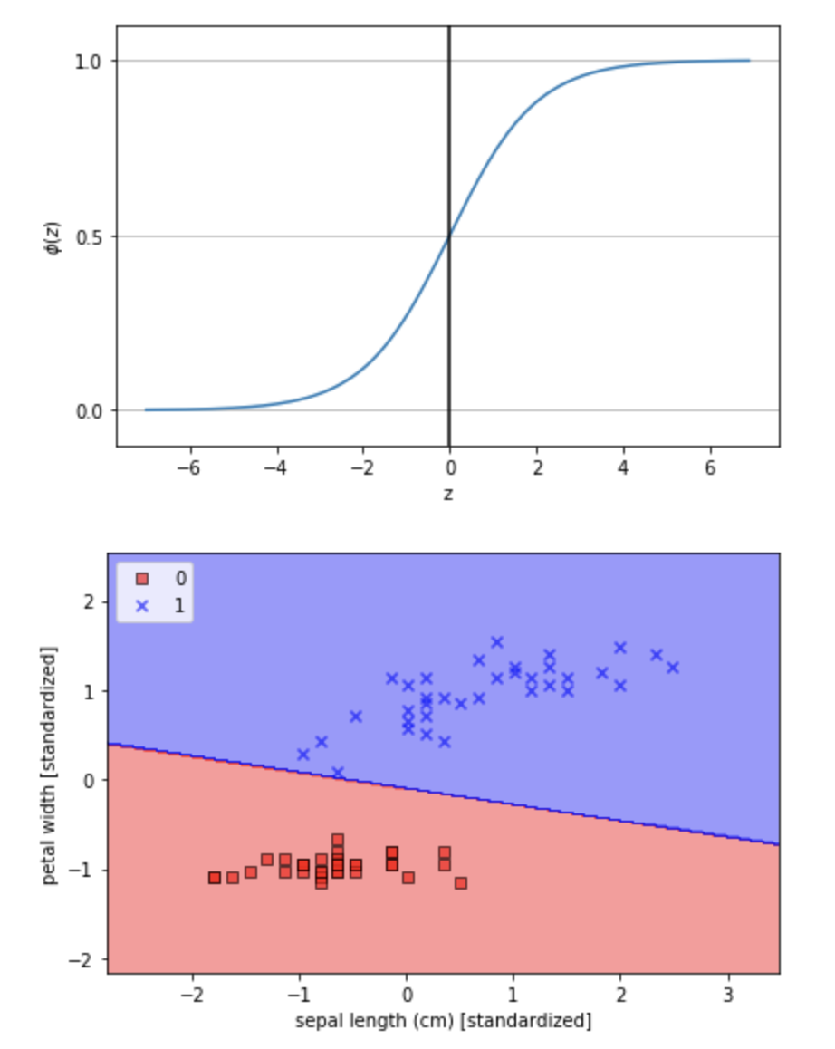
總結Logistic Regression好處資料不需要線性可分並且可以獲得機率，但從圖可發現前兩天的SVM方法可以找到更好的線。認識了感知器與邏輯斯回歸後明天就來學Decision Tree還有Random Forest～