昨天介紹完Linear Regression，今天要來繼續介紹高斯函數在Linear-Regression的應用。高斯函數本身不是SKlearn中的模組，因此，需要自己編寫一個自訂的高斯函式：

• 首先，匯入sklearn.base中的估算器BaseEstimator、轉換器TransformerMixin

sklearn.base.BaseEstimator詳細可以參考(官方文件)：http://scikit-learn.org/stable/modules/generated/sklearn.base.BaseEstimator.html

from sklearn.base import BaseEstimator, TransformerMixin
from sklearn.linear_model import LinearRegression
from sklearn.pipeline import make_pipeline

• 再來，自定義GaussianFeatures函數。

class GaussianFeatures(BaseEstimator, TransformerMixin):
    """Uniformly spaced Gaussian features for one-dimensional input"""
    
    def __init__(self, N, width_factor=1.0):
        self.N = N
        self.width_factor = width_factor
    
    @staticmethod
    def _gauss_basis(x, y, width, axis=None):
        arg = (x - y) / width
        return np.exp(-0.5 * np.sum(arg ** 2, axis))
        
    def fit(self, X, y=None):
        # create N centers spread along the data range
        self.centers_ = np.linspace(X.min(), X.max(), self.N)
        self.width_ = self.width_factor * (self.centers_[1] - self.centers_[0])
        return self
        
    def transform(self, X):
        return self._gauss_basis(X[:, :, np.newaxis], self.centers_,
                                 self.width_, axis=1)
    
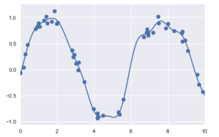
gauss_model = make_pipeline(GaussianFeatures(20),
                            LinearRegression())
gauss_model.fit(x[:, np.newaxis], y)
yfit = gauss_model.predict(xfit[:, np.newaxis])

plt.scatter(x, y)
plt.plot(xfit, yfit)
plt.xlim(0, 10);

• 利用自訂的高斯函數，將資料映射到30-dimensional basis中。

def basis_plot(model, title=None):
    fig, ax = plt.subplots(2, sharex=True)
    model.fit(x[:, np.newaxis], y)
    ax[0].scatter(x, y)
    ax[0].plot(xfit, model.predict(xfit[:, np.newaxis]))
    ax[0].set(xlabel='x', ylabel='y', ylim=(-1.5, 1.5))
    
    if title:
        ax[0].set_title(title)

    ax[1].plot(model.steps[0][1].centers_,
               model.steps[1][1].coef_)
    ax[1].set(xlabel='basis location',
              ylabel='coefficient',
              xlim=(0, 10))
    
model = make_pipeline(GaussianFeatures(30), LinearRegression())
basis_plot(model)

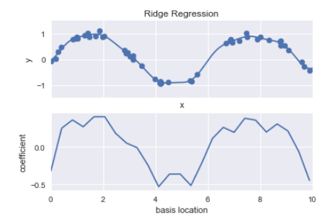
可以在basis_plot中，看到當基函數重疊時，會發生過度擬合(over-fitting)的狀況，因此，我們要限制這些尖峰值得出現，有以下幾種方式：

• Ridge regression
  最常見的正規化方式，亦稱為Tikhonov regularization，這個正規方式利用系數的平方和(2-norms)，公式如下：
  
  其中，是控制函數產生極端值強度的參數。

from sklearn.linear_model import Ridge
model = make_pipeline(GaussianFeatures(25), Ridge(alpha=0.1))
basis_plot(model, title='Ridge Regression')

• Lasso regression
  第二種正規化方式，是把第一種方式的回歸係數原本用平方和處理轉換為取絕對值的和，其公式如下：
  

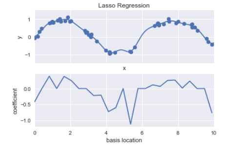
from sklearn.linear_model import Lasso
model = make_pipeline(GaussianFeatures(25), Lasso(alpha=0.001))
basis_plot(model, title='Lasso Regression')