昨天介紹完貝氏分類器(Bayes Classification)，有沒有覺得SKlearn內的函數真的很好用呀!今天要來介紹常用的線性迴歸(Linear-Regression)。

Linear Regression

線性回歸簡單來說，就是將複雜的資料數據，擬和至一條直線上，就能方便預測未來的資料。

import matplotlib.pyplot as plt
import seaborn as sns; sns.set()
import numpy as np

先從簡單的線性回歸舉例， ， 稱為斜率， 稱為截距。

• 考慮到使用的數據，如下所舉例斜率為3，截距為-5。

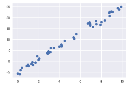
rng = np.random.RandomState(1)
x = 10 * rng.rand(50)
y = 3 * x - 5 + rng.randn(50)
plt.scatter(x, y);

• 再來，使用SKlearn中的LinearRegression模組來擬合數據，並利用plt.plot()方式建構繪製出最適合的線。

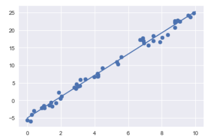
from sklearn.linear_model import LinearRegression
model = LinearRegression(fit_intercept=True)

model.fit(x[:, np.newaxis], y)

xfit = np.linspace(0, 10, 1000)
yfit = model.predict(xfit[:, np.newaxis])

plt.scatter(x, y)
plt.plot(xfit, yfit);

• 而模型的斜率及截距，分別儲存在model.coef_[0] 和 model.intercept_中。

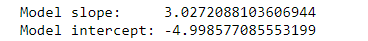
print("Model slope:    ", model.coef_[0])
print("Model intercept:", model.intercept_)

• Multidimensional linear models
  多維回歸的線性模型， ，可以在y上建立多維的陣列。

rng = np.random.RandomState(1)
X = 10 * rng.rand(100, 3)
y = 0.5 + np.dot(X, [1.5, -1., 2.])

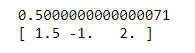
model.fit(X, y)
print(model.intercept_)
print(model.coef_)

Polynomial basis functions

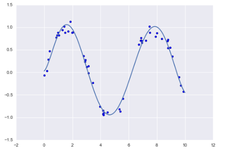
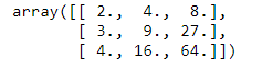
利用SKlearn中匯入 PolynomialFeatures，來做多項式函數處理。

from sklearn.preprocessing import PolynomialFeatures
x = np.array([2, 3, 4])
poly = PolynomialFeatures(3, include_bias=False)
poly.fit_transform(x[:, None])

• 並且利用make_pipeline，一維陣列轉換為三維陣列，加入線性回歸中。

from sklearn.pipeline import make_pipeline
poly_model = make_pipeline(PolynomialFeatures(7), LinearRegression())

• 轉換完成後，可以看到(x,y)的關係為正弦圖形

rng = np.random.RandomState(1)
x = 10 * rng.rand(50)
y = np.sin(x) + 0.1 * rng.randn(50)

poly_model.fit(x[:, np.newaxis], y)
yfit = poly_model.predict(xfit[:, np.newaxis])

plt.scatter(x, y)
plt.plot(xfit, yfit);