今天要來介紹支持向量機(Support Vector Machines,SVM)，我覺得它是最方便、好用的監督式演算法，主要可以用來做模式辨識、分群、回歸的機器學習。

• 首先，先匯入今天所需的模組及資料集合

%matplotlib inline
import numpy as np
import matplotlib.pyplot as plt
from scipy import stats

# use seaborn plotting defaults
import seaborn as sns; sns.set()

• 建立資料，建立資料點的個數：n_samples、分為幾個類別的資料：centers

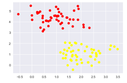
from sklearn.datasets.samples_generator import make_blobs
X, y = make_blobs(n_samples=100, centers=2,
                  random_state=0, cluster_std=0.60)
plt.scatter(X[:, 0], X[:, 1], c=y, s=50, cmap='autumn');

• 再來，就需要用直線來分割兩個不同類別的資料。

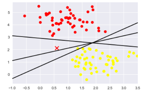
xfit = np.linspace(-1, 3.5)
plt.scatter(X[:, 0], X[:, 1], c=y, s=50, cmap='autumn')
plt.plot([0.6], [2.1], 'x', color='red', markeredgewidth=2, markersize=10)

for m, b in [(1, 0.65), (0.5, 1.6), (-0.2, 2.9)]:
    plt.plot(xfit, m * xfit + b, '-k')

plt.xlim(-1, 3.5);

• Maximizing the Margin
  在資料分群，我們應該要更明確的分群平面上不同類別的點，因此繪製一些有寬度的邊，"直到最近的點"：

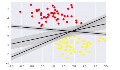
xfit = np.linspace(-1, 3.5)
plt.scatter(X[:, 0], X[:, 1], c=y, s=50, cmap='autumn')

for m, b, d in [(1, 0.65, 0.33), (0.5, 1.6, 0.55), (-0.2, 2.9, 0.2)]:
    yfit = m * xfit + b
    plt.plot(xfit, yfit, '-k')
    plt.fill_between(xfit, yfit - d, yfit + d, edgecolor='none',
                     color='#AAAAAA', alpha=0.4)

plt.xlim(-1, 3.5);

Fitting a support vector machine

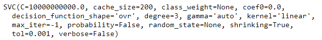
擬合支持向量機，可以看一下這個數據的實際擬合結果，使用Scikit-Learn的支持向量分類器來訓練這個數據的SVM模型：

from sklearn.svm import SVC # "Support vector classifier"
model = SVC(kernel='linear', C=1E10)
model.fit(X, y)

• 為了在平面上更清楚的呈現資料分群後的邊界，在這邊自行定義plot_svm_decision_function()，實線到虛線的部分代表可能會造成over-fitting的情況

def plot_svm_decision_function(model, ax=None, plot_support=True):
    """Plot the decision function for a 2D SVC"""
    if ax is None:
        ax = plt.gca()
    xlim = ax.get_xlim()
    ylim = ax.get_ylim()
    
    # create grid to evaluate model
    x = np.linspace(xlim[0], xlim[1], 30)
    y = np.linspace(ylim[0], ylim[1], 30)
    Y, X = np.meshgrid(y, x)
    xy = np.vstack([X.ravel(), Y.ravel()]).T
    P = model.decision_function(xy).reshape(X.shape)
    
    # plot decision boundary and margins
    ax.contour(X, Y, P, colors='k',
               levels=[-1, 0, 1], alpha=0.5,
               linestyles=['--', '-', '--'])
    
    # plot support vectors
    if plot_support:
        ax.scatter(model.support_vectors_[:, 0],
                   model.support_vectors_[:, 1],
                   s=300, linewidth=1, facecolors='none');
    ax.set_xlim(xlim)
    ax.set_ylim(ylim)

plt.scatter(X[:, 0], X[:, 1], c=y, s=50, cmap='autumn')
plot_svm_decision_function(model);

• 在上圖繪製邊界，有一些訓練的點會觸及邊界，這些擬合的關鍵元素，SKlearn就會儲存至support_vectors_ 中

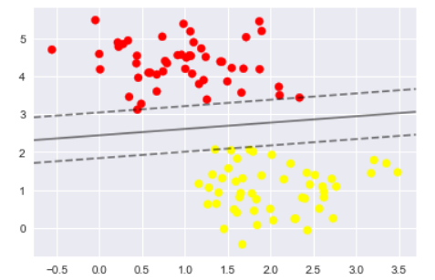
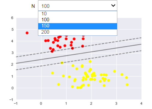
model.support_vectors_

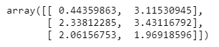
在上圖中，我們可以知道，幫點未觸及邊界線，就不會有over-fitting的情況，再來用前[80/200]的資料集

def plot_svm(N=10, ax=None):
    X, y = make_blobs(n_samples=200, centers=2,
                      random_state=0, cluster_std=0.60)
    X = X[:N]
    y = y[:N]
    model = SVC(kernel='linear', C=1E10)
    model.fit(X, y)
    
    ax = ax or plt.gca()
    ax.scatter(X[:, 0], X[:, 1], c=y, s=50, cmap='autumn')
    ax.set_xlim(-1, 4)
    ax.set_ylim(-1, 6)
    plot_svc_decision_function(model, ax)

fig, ax = plt.subplots(1, 2, figsize=(16, 6))
fig.subplots_adjust(left=0.0625, right=0.95, wspace=0.1)
for axi, N in zip(ax, [80, 200]):
    plot_svm(N, axi)
    axi.set_title('N = {0}'.format(N))

• 也可以利用interact()，動態查詢資料及的情況。

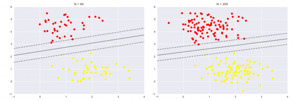
from ipywidgets import interact, fixed
interact(plot_svm, N=[10,100,150,200], ax=fixed(None));