網路上有許多介紹VAE的文章與影片,但許多解釋公式都無法得知為什麼,但這也是個人對於看paper的功力太差所以才能努力爬文觀看他人解析,而最後終於找到一個合乎我疑問的解釋[1],最後也發現[2]的解釋方法就是利用[1]來去推導,最終解開了我的為甚麼。
機率公式1
機率公式2
20190706更新:
從[4]得知,假設平常訓練模型輸入為X,輸出一個類別Y,則我們會建立一個模型f(X;W),使得輸入X輸出Y的機率最大,即是p(Y|X)最大。
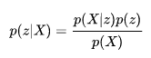
而若想使用生成模型,則必須轉為貝葉斯公式,如下圖(z=Y)。這裡X為觀測變量意旨容易觀察到X,z為隱藏變量意旨不易觀察,於是我們需要知道z的隱藏變量就可使用貝葉斯公式求解。
而p(z)的z機率能由我們決定,而較難解決的則是p(X|z),這能使用最大似然估計解這個參數。
來源[4]。
但若隱藏變量是一個連續機率分布的空間,公式如下圖,分母意思是一個連續機率為隱藏變量z輸出X的機率乘上z的機率,而這在數學上要求導是有難度的。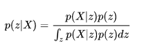
來源[4]。
簡單來說求解最大似然估計在一個高維空間裡要去解這個公式就不那麼容易。而重要的是最後要去度量與p(z|X)的差異,但這裡我們並不知道X的真實分布是什麼(另一篇文章是用p(x)來解說)。
然而不管是要近似文章一的p(x)或是文章二的p(z|X)只要知道最後我們都必須去度量與真實分布差異,所以迴避計算高維的問題最後VAE當中使用一個機率分布q(z)來逼近p(z|X)或p(x)。
在這裡先驗機率可以想像成是一個真實存在的,但我們無法得知他真實的機率是多少,而後驗機率則是在某個事件當中發生另一個事件的機率是多少,而在VAE當中就能利用這特性去近似函數(實際上要最大似然)。
主要是先驗機率是存在的我們無法去控制,若可控制則會改變原先的結果,但後驗則可想像成一個類似映射的方式,多添加一個可控制的機率函數產生出原先的真實的機率。而這邊使用貝葉斯則可轉換為這樣的構思。
首先將上述貝葉斯公式轉換為文字敘述,使得快速理解。
[6]提到後驗與先驗使用貝葉斯公式則
比例P(B|A)/P(B)也有時被稱作標准似然度(standardised likelihood),貝氏定理可表述為:
後驗概率 = 標准似然度*先驗概率
在上述中可得知雖然很難計算出最大似然數,但可以假設一個q(z),而p(z|X)是後驗機率,則只要使用KL散度最小化q(z)與p(z|x)即可。(只要Encoder輸出的z是高斯分布就足夠了)
首先介紹ELBO,其中有使用到貝葉斯(可看成一般機率公式轉換),這裡使用一個q(z)趨近p(z|x),而使用的度量方式為KL散度,KL散度即是兩者分布的差異。但我們無法直接求min,因為我們無法得知p(x)的真實分布情況只知道它是存在的,如下圖的推導。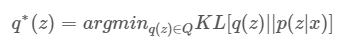
公式,來源[1]。
1.KL散度指數乘法轉為減法。
2.p(z|x)轉換貝葉斯公式。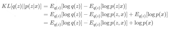
推導,來源[1]。
但可將上述公式轉換為ELBO進行推導。如下圖。
1.p(x)扣掉上述推導後公式,原先的p(x)就消失了,這動作主要為了後面繼續推導。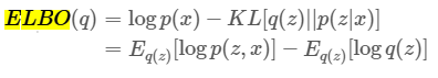
來源[1]。
你會好奇為何可以直接扣除logp(x),首先觀看[1]的說法
- 由于logp(x)相对于q(z)是一个常量,而我们想要最小化KL,ELBO等于负的KL加上一个常量,所以我们最大化ELBO就等价于最小化KL。
- 最大化logp(x)就是对观测数据的极大似然估计(即log evidence),由于KL是非负的,所以这个目标函数是极大似然估计的下确界(即evidence lower bound, ELBO)。
簡單來說我們要最小化q(z)(微分),而logp(x)它不依賴z(微分是常數)所以在這裡可視為常量,那最小化KL即是最大化ELBO,因ELBO=常量-KL,KL越小ELBO越大。接著繼續推導化簡為如下。
1.p(z,x)機率公式轉換為p(x|z)p(z)。
2.指數關係,乘法變加法。
3.後兩項轉為KL。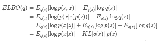
來源[1]。
最後這公式沒有了計算p(x)分布,而是用一個隱變量z來近似x,而在VAE當中這隱變量都假設為方差為1平均為0。
這裡介紹兩種方法,方法一來自[2],方法二則是使用上面公式帶入,方法一其實與方法二很像,但方法一有些數學公式沒很熟悉則會轉不過來。因此將上述介紹的公式直接使用在上面會更加清晰。
作者使用聯合機率分布,以機率來說則在計算同時產生x和z的機率,Z是一個隱藏變量(簡單來說就是Encoder後的輸出),q(X,Z)則是一個近似p(X,Z),最後面則會直接假設Z輸出是方差=1、均值=0的二維高斯變量。
假設q(x, z)是一個度量p(x, z)的聯合機率分布,使用KL散度進行度量計算,如下圖。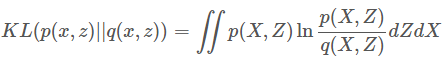
來源[2]。
1.將p(x,z)使用機率轉換公式轉為p(x)p(z|x)。
2.轉為期望值公式。
3.將右邊公式p(x)乘法轉為加法。
4.分開為左右兩式。
5.左式直接對Z做微分,可以看到Z為一個輸出乘上p(x)所以結果為p(x)。([2]解釋為左式因p(x)與dz無關所以提出)。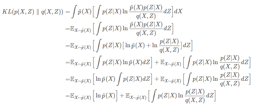
來源[2]。
[2]解說為,lnp(x)雖然是一個複雜的分布,雖然無法求出但可確定它是存在,所以可當作一常數。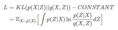
來源[2]。
1.q(x,z)轉為q(x|z)q(z)。
2.將右式q(x|z)提出。
3.轉為期望公式。
4.右式轉為KL。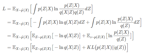
來源[2]。
為了驗證[1]所以使用上述ELBO求出。假設q(z)近似p(z|X)。
1.展開KL散度。
2.提出q(z)。
3.logp(z|X)使用貝葉斯轉換。
4.將與z無關的項提出,logp(x)。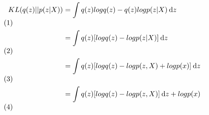
將logp(x)移置左項,最小化KL等於最大化ELBO。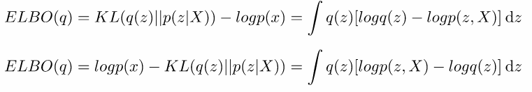
1.帶入上述推導公式。
2.logp(z,X)使用機率公式轉為logp(X|z)p(z)。
3.提出logp(z),指數乘法等於加法。
4.將q(z)和p(z)轉為KL。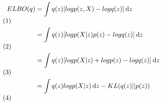
接著要將最後推倒結果給展開,這裡延續方法一[2]。
對於KL項假設q(z)是個正態分布,方差=1、均值=0,這裡公式基本上都是KL展開化簡,有興趣可前往詳細KL多維高斯分布推導。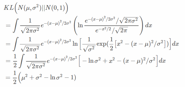
來源[2]。
論文使用了兩種分布,其第一種結果為交叉熵,第二種為均方誤差。
第一種
使用伯努利分布,如下。
1.將每個維度的機率帶入伯努利分布。
2.連乘轉為指數運算。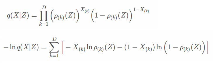
來源[2]。
結果即是交叉熵。這裡要注意的是ρ(z)是Decoder運算,因伯努利分布所以輸出資料必須在0~1,可用sigmoid函數實現。
第二種
使用正態分布,而這裡與上述正態分布推導相同。
1.帶入正態分布。
2.連乘轉為指數運算。
3.固定方差為常數,因固定方差所以後向可無視,而平方中的alpha可提出。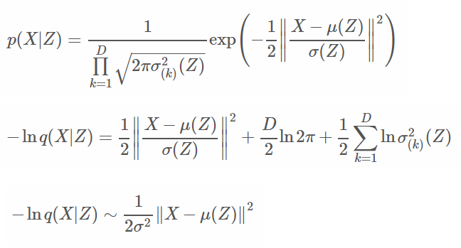
這裡的程式碼與AutoEncoder很像,差別在於Encoder和loss不同。
learning_rate: 學習率。
batch_size: 批次訓練數量。
train_times: 訓練次數。
train_step: 驗證步伐。
encoder_hidden: 編碼神經網路隱藏層數量。
decoder_hidden: 解碼神經網路隱藏層數量。
output_size: 編碼輸出數量。
learning_rate = 0.001
batch_size = 128
train_times = 200
train_step = 1

encoder_hidden1_size = 500
encoder_hidden2_size = 300
encoder_hidden3_size = 150
decoder_hidden1_size = 150
decoder_hidden2_size = 300
decoder_hidden3_size = 500

output_size = 2
批量歸一化
之前有介紹,可前往網址觀看。
def layer_batch_norm(x, n_out, is_train):
    beta = tf.get_variable("beta", [n_out], initializer=tf.zeros_initializer())
    gamma = tf.get_variable("gamma", [n_out], initializer=tf.ones_initializer())

    batch_mean, batch_var = tf.nn.moments(x, [0], name='moments')
    ema = tf.train.ExponentialMovingAverage(decay=0.9)
    ema_apply_op = ema.apply([batch_mean, batch_var])

    def mean_var_with_update():
        with tf.control_dependencies([ema_apply_op]):
            return tf.identity(batch_mean), tf.identity(batch_var)

    mean, var = tf.cond(is_train, mean_var_with_update, lambda:(batch_mean, batch_var))

    x_r = tf.reshape(x, [-1, 1, 1, n_out])
    normed = tf.nn.batch_norm_with_global_normalization(x_r, mean, var, beta, gamma, 1e-3, True)
    return tf.reshape(normed, [-1, n_out])
神經網路層
def layer(x, weights_shape, activation='relu'):
    init = tf.random_normal_initializer(stddev=np.sqrt(2. / weights_shape[0]))
    weights = tf.get_variable(name="weights", shape=weights_shape, initializer=init)
    biases = tf.get_variable(name="biases", shape=weights_shape[1], initializer=init)
    mat_add = tf.matmul(x, weights) + biases
    #mat_add = layer_batch_norm(mat_add, weights_shape[1], tf.constant(True, dtype=tf.bool))

    if activation == 'relu':
        output = tf.nn.relu(mat_add)
    elif activation == 'sigmoid':
        output = tf.nn.sigmoid(mat_add)
    elif activation == 'softplus':
        output = tf.nn.softplus(mat_add)
    else:
        output = mat_add
    return output
這裡輸出兩個向量,一個為標準差,一個為均值,依照原先構思乘上一個正態分布。而很多人也會將標準差先改為ln(std^2),但這裡使用上述推導公式標準差實作。
def encoder(x):
    with tf.variable_scope("encoder"):
        with tf.variable_scope("hide1"):
            hide1 = layer(x, [784, encoder_hidden1_size], activation='softplus')
        with tf.variable_scope("hide2"):
            hide2 = layer(hide1, [encoder_hidden1_size, encoder_hidden2_size], activation='softplus')
        with tf.variable_scope("hide3"):
            hide3 = layer(hide2, [encoder_hidden2_size, encoder_hidden3_size], activation='softplus')
        with tf.variable_scope("mean"):
            mean = layer(hide3, [encoder_hidden3_size, output_size], activation=None)
        with tf.variable_scope("std"):
            log_var = layer(hide3, [encoder_hidden3_size, output_size], activation=None)
        with tf.variable_scope("output"):
            eps = tf.random_normal(shape=tf.shape(log_var), mean=0, stddev=1, dtype=tf.float32)
            # log_var = ln(std^2)
            #output = mean + tf.exp(log_var) * 0.5 * eps
            # log_var = std
            output = mean + log_var * eps
    return output, mean, log_var
def decoder(x):
    with tf.variable_scope("decoder", reuse=tf.AUTO_REUSE):
        with tf.variable_scope("hide1", reuse=tf.AUTO_REUSE):
            hide1 = layer(x, [output_size, decoder_hidden1_size], activation='softplus')
        with tf.variable_scope("hide2", reuse=tf.AUTO_REUSE):
            hide2 = layer(hide1, [decoder_hidden1_size, decoder_hidden2_size], activation='softplus')
        with tf.variable_scope("hide3", reuse=tf.AUTO_REUSE):
            hide3 = layer(hide2, [decoder_hidden2_size, decoder_hidden3_size], activation='softplus')
        with tf.variable_scope("output", reuse=tf.AUTO_REUSE):
            output = layer(hide3, [decoder_hidden3_size, 784], activation='sigmoid')
    return output
def predict(x):
    output, mean, log_var = encoder(x)
    return decoder(output), mean, log_var
依照上述推導公式帶入,若再Encoder使用ln(std^2)則要使用註解公式。
def loss(output, x, mean, log_var):
    cross_loss = -tf.reduce_sum(x * tf.log(output + 1e-8) + (1 - x) * tf.log(1 - output + 1e-8), 1)
    cross_mean_loss = tf.reduce_mean(cross_loss)
    # log_var = ln(std^2)
    #kl_loss = 0.5 * tf.reduce_sum(tf.square(mean) + tf.exp(log_var) - log_var - 1, axis=1)

    # log_var mean std
    kl_loss = 0.5 * tf.reduce_sum(tf.square(mean) + tf.square(log_var) - tf.log(tf.square(log_var)) - 1, axis=1)
    kl_mean_loss = tf.reduce_mean(kl_loss)
    loss = cross_mean_loss + kl_mean_loss
    loss_his = tf.summary.scalar("loss", loss)
    return loss
def train(loss, index):
    return tf.train.AdamOptimizer(learning_rate=learning_rate, beta1=0.9, beta2=0.999, epsilon=1e-08).minimize(loss, global_step=index)
    #return tf.train.RMSPropOptimizer(learning_rate, decay=0.9).minimize(loss,
    #global_step=index)
    #return tf.train.AdagradOptimizer(learning_rate).minimize(loss,
    #global_step=index)
    #return tf.train.MomentumOptimizer(learning_rate,
    #momentum=0.9).minimize(loss, global_step=index)
    #return tf.train.GradientDescentOptimizer(learning_rate).minimize(loss,
    #global_step=index)
def image_summary(label, image_data):
    reshap_data = tf.reshape(image_data, [-1, 28, 28, 1])
    tf.summary.image(label, reshap_data)

def accuracy(output, t):
    image_summary("input_image", t)
    image_summary("output_image", output)
    sqrt_loss = tf.sqrt(tf.reduce_sum(tf.square(tf.subtract(output, t)), 1))
    y = tf.reduce_mean(sqrt_loss)
    tf.summary.scalar("accuracy error", y)

    return y
1.初始化資料。
2.預測函數。
3.損失函數。
4.訓練函數。
5.驗證函數。
6.tensorboard可視化。
7.開始訓練。
8.輸出q(X|z)結果。
if __name__ == '__main__':
    # init
    mnist = input_data.read_data_sets("MNIST/", one_hot=True)
    input_x = tf.placeholder(tf.float32, shape=[None, 784], name="input_x")

    # predict
    predict_op, mean, log_var = predict(input_x)

    # loss
    loss_op = loss(predict_op, input_x, mean, log_var)

    # train
    index = tf.Variable(0, name="train_time")
    train_op = train(loss_op, index)

    # accuracy
    accuracy_op = accuracy(predict_op, input_x)

    # graph
    summary_op = tf.summary.merge_all()
    session = tf.Session()
    summary_writer = tf.summary.FileWriter("log/", graph=session.graph)

    data_x = tf.placeholder(tf.float32, shape=[None, output_size], name="data_x")
    decoder_op = decoder(data_x)

    init_value = tf.global_variables_initializer()
    session.run(init_value)

    for time in range(train_times):
        avg_loss = 0.
        total_batch = int(mnist.train.num_examples / batch_size)
        for i in range(total_batch):
            minibatch_x, _ = mnist.train.next_batch(batch_size)
            session.run(train_op, feed_dict={input_x: minibatch_x})
            avg_loss += session.run(loss_op, feed_dict={input_x: minibatch_x}) / total_batch

        if (time + 1) % train_step == 0:
            accuracy = session.run(accuracy_op, feed_dict={input_x: mnist.validation.images})
            summary_str = session.run(summary_op, feed_dict={input_x: mnist.validation.images})
            summary_writer.add_summary(summary_str, session.run(index))
            print("train times:", (time + 1),
                        " avg_loss:", avg_loss,
                        " accuracy:", accuracy)

    # make to size 20 * 20 images form q(z) of distributed
    imgs = np.empty((28 * 20, 28 * 20))
    index_x = 0
    for x in range(-10,10,1):
        index_y = 0
        for y in range(-10,10,1):
            value = np.array([[float(x / 5.), float(y / 5.)]])
            img = session.run(decoder_op, feed_dict={data_x:value})
            imgs[index_x * 28:(index_x + 1) * 28, index_y * 28:(index_y + 1) * 28] = img.reshape((28, 28))
            index_y += 1
        index_x += 1

    plt.imshow(imgs, cmap=plt.get_cmap('gray'))
    plt.show()

    session.close()
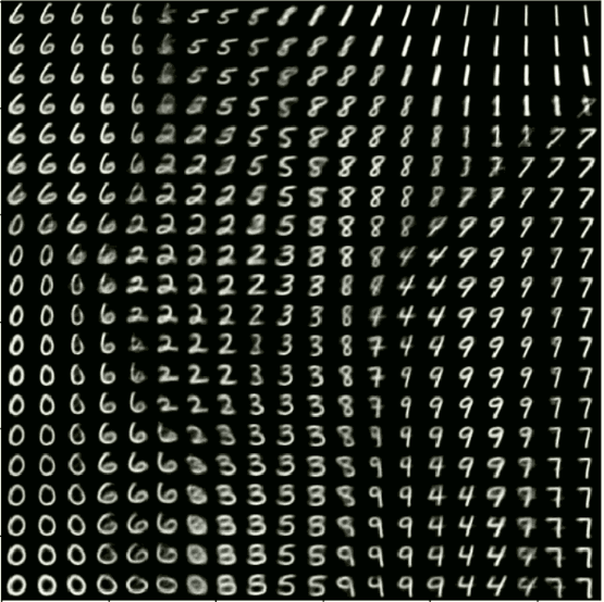
其實VAE整體上的公式理解並不算太複雜,而其實VAE最理想是求最大似然數,但因連續機率難以求出只好使用趨近方式,最後產生出的結果圖片都是有些模糊的,可能是因為高斯分布的關係(在影像處理中的模糊也是其中用法),接著介紹GAN,它可以使圖片更加清晰的呈現,就讓我們期待GAN會帶來什麼不同的驚喜吧。
補充:若對其中如何使用正態分布產生的圖有興趣可觀看李弘毅老師的ML Lecture 18觀看,裡面也有另一個想法的公式推導。
另外這網站也有正態分布圖片能觀看,裡面也是有不同的想法的公式推導。
[1]cairohy(2018) 变分推断(一):介绍变分推断 from: http://cairohy.github.io/2018/02/28/vi/VI-1/
[2]qixinbo(2018) 变分自编码器的原理和程序解析from: https://qixinbo.info/2018/07/24/vae/
[3]維基百科(2018) 相對熵 from: https://zh.wikipedia.org/wiki/%E7%9B%B8%E5%AF%B9%E7%86%B5
[4]冯超(2017) VAE(2)——基本思想 from: https://zhuanlan.zhihu.com/p/22464764
[5]极大似然估计详解(2017) 知行流浪 from: https://blog.csdn.net/zengxiantao1994/article/details/72787849
[6]維基百科(2018) 貝氏定理from: https://zh.wikipedia.org/wiki/%E8%B4%9D%E5%8F%B6%E6%96%AF%E5%AE%9A%E7%90%86
 Kevin
Kevin

 iThome鐵人賽