前言

Monte Carlo Method需要等到整個episode跑完才能更新，如果episode需要很多step才能結束的話會怎樣？如果你拿Monte Carlo去跑Taxi環境的話，會發現需要跑很久。這是因為我們State與Action太多，再加上隨機策略要到達Final State需要相當多step，進而造成更新很慢。

我們可以引進dynamic programming裡bootstrapping的概念，每個state只須依據下個state的值來更新，就不用等到episode跑完浪費時間了。

這種Monte Carlo裡的sample概念與dynamic programming裡的bootstrapping概念一起使用的算法就稱為時序差分學習 (Temporal difference learning)，簡稱TD Learning。

時序差分學習 (Temporal difference learning)

我們先從Monte Carlo來看，Monte Carlo的更新方法很簡單，依照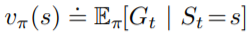來更新Value。

期望值可以用平均來計算，所以可以寫成

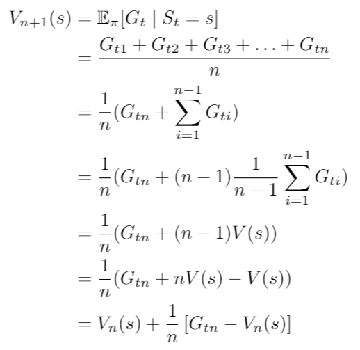
這邊用表示目前考慮幾次，為考慮n個不同的之平均。

這就是前天結尾說的用incremental取代平均值，可以把的部分可以換成任意值，稱為step-size或learning rate，通常以表示。

這種方法的好處是越後面的資訊不會被前面的資訊稀釋。舉例來說，假如環境是會變動的，如果我們step-size用原本的的話，環境變動後我們得到的對期望值的影響會隨著變大而越來越小。如果將step-size設為常數，變動後的都會有固定比例來改變期望值的值。

所以Monte Carlo公式可以寫成這樣：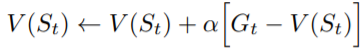

這邊就不特別把的寫出來了，但實際上一樣是根據每個的值來增加

還記得的期望值嗎？

我們可以將以上面期望值的形式取代，形成期望值的期望值，這種更新方法就稱為Temporal difference learning。

可以證明TD Learning一樣可以收斂，且理論上收斂的速度比Monte Carlo還要快

公式中稱為TD error，可以想成我們目前的估計值與真實值的差距。當差距越大，的更新越多，當差距越小，的更新就越少。

事實上，Monte Carlo Method就是一種多步更新的TD Learning，可以從Monte Carlo的error看到；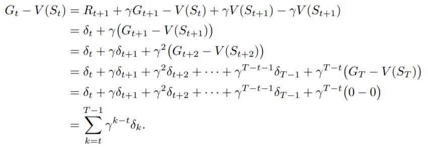

Monte Carlo的error其實就是TD error的總和，也就是將TD Learning延伸到整個episode在算error來更新，更多細節會在之後的n-step TD learning提到。

TD Learning一樣可以視為一種GPI的形式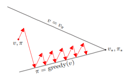

其中，更新Value的部分就是用上面的更新，而Policy一樣以-greedy的方式更新(因為要持續exploration)，最後就能找到最佳解。

總結

了解TD Learning的更新方式後，明天就可以直接來實作兩種TD Learning的演算法：Sarsa與Q Learning，與他們的變形。學會這兩個演算法後，就可以解決在有限state裡大部分的Reinforcement Learning問題了！