很多常見的強化學習算法都是根據貝爾曼方程來的,我們可以把強化學習的目標,用Value Function來表示。之後我們只要求這個Value Function的解就能間接找到強化學習的最佳解,而要求Value Function的解,就必須經過貝爾曼方程來簡化它!!
先來看兩種強化學習的環境
Episodic Tasks表示環境中必須存在Final State,只要時間夠久,最後一定可以結束。我們稱這從開始到結束為1個Episode。像是棋盤遊戲,或是走迷宮等等。
而Continuing Tasks就是除了Episodic Tasks以外的所有Task,或著可以想像成到還無法終止的環境。
可以透過自行定義改變環境的種類,像是我們常會把Continuing Task設定跑固定個時間點後結束,就成了Episodic Tasks
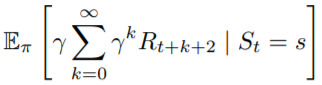
現在我們來用數學公式描述之前提到的強化學習的目標,我們說過最大化的目標必須是時間點之後的Reward總和,我們稱這個目標為Expected return,用符號G來表示:
,
表示在時間點
,
則表示最後Final State的時間點。
可以看到Continuing Tasks不滿足上面這個公式,因為的話
就不會收斂,所以我們引進一個衰減值
,
的用途除了讓Continuing Tasks收斂外,也能表示對未來的重視程度。
越高,表示考慮到的未來越多,
越低,表示越重視眼前的目標。
從更新後的Expected return來看:對
的影響可以從下面兩個極端值理解:
而環境對範圍的影響如下:
Policy是用來表示我們Agent在某狀態下行為的機率,符號為。其本質上就是一個從State映射到Action上的函數。從機率形式上比較容易理解:
表示在
這個State上,做行為
的機率。
可以從下面的圖來看:
現在Agent在圖中的位置,有4個行為(Left, Right, Top, Down)。現在Agent的policy為隨機策略,選擇Left, Right, Top, Down的機率皆為25%,所以
的機率分布為以下四種:
我們重新來看一下Expected Return的定義,在某個時間點後的Reward總和。好像哪裡怪怪的?每個時間點
所在的State可能都不一樣,而Action又必須根據State來選擇,那怎麼能只用時間
的Return來當作目標勒?所以我們用一個新的Function來表示在某個State底下的Expected Return,這個Function稱為價值函數(Value Function),可以寫作:
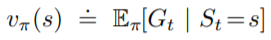
底下有一個
用來表示這個function是依據策略
來決定值的。
另外,為了方便計算,我們可以對每個行為都算它的價值函數,稱為動作價值函數 (Action-Value Function),表示為:
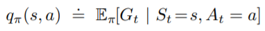
一樣用來表示這個function是依照策略
來決定
可以看出來,Value Function其實就是Action-Value Function的和:
這邊推導看過就好,結果比較重要
把展開
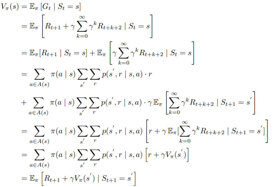
這邊
因篇幅關係沒有加上集合範圍,可以參考底部公式的範圍,
前方的
只是方便理解,實際上可用上方講的
取代
先把根據定義的公式拆開,再把期望值分為兩部分。
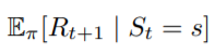
第一部分根據期望值的定義展開,這邊的隨機變數為且機率為
,依照昨天最後講的公式,可以得到
。
接著根據期望值的定義:隨機變數*對應隨機變數出現的機率,得到。
最後我們是計算在策略下的值,每一個Action都有固定的比例對這個State上的Value做出貢獻,我們可以想成每一個Action對這個期望值有一定的權重。以上面迷宮例子來看,有25%的Reward是從
來的;有25%的Reward是從
,以此類推。所以必須對每個Action都乘上Policy佔的比例。
第二部分跟上面很像,差別在於這邊期望值裡的隨機變數為,我們可以仿造第一部分的公式展開,你會發現式子中的
會根據下一個State的不同而改變。我們可以只專注在下一個State與它的機率,剩下部分就留給下下一個State去考慮就好。所以我們用下個State的期望值來解決
不同的問題,但要記得我們需要考慮下個State的所有可能。
仔細看第二部分,其實就是原式在時的情形,所以把它換成
最後把同項的合在一起,再寫成期望值的定義就好了。
這個公式就叫做貝爾曼方程(Bellman Function),仔細看它的結構,原本我們需要算時間點~
的Return,這是件非常麻煩的事,你要記錄每個時間點
的Return值,並且要等到return收斂後才能更新。但是Bellman Function將所有State的關係壓縮為只跟後一個State有關,這種不需要等return收斂就能更新的方法稱為Bootstrapping。
有的Bellman Function形式,當然也有
的形式
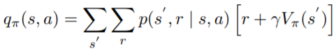
可以看到Action-Value的Bellman Function只是把的
部分拿掉,這是因為Action-value已經選擇特定的Action,其他Action對期望值的影響都為0,因為不可能會選到除了
以外的Action。
看數學式子看到眼睛快花掉,明天終於要寫Code啦XD
Bellman Function可以很有效率地減少運算所需的記憶體,接來下我們就可以求出Bellman Function的解,根據這個解來找出最佳策略!