iT邦幫忙

第 12 屆 iThome 鐵人賽

DAY 25
1
AI & Data

Knock Knock! Deep Learning系列 第 25

Day 24 / DL x RL / 決策與 RL

  • 分享至 

  • xImage
  •  

結束了 CV 子系列,接下來要來介紹完全不同於 supervised / unsupervised learning 的訓練方法 —— reinforcement learning(RL,強化學習)

2013 年 Google DeepMind 團隊發表遊戲 Atari 基於 DL 和 RL 訓練出能打敗人類的 AI,也是 DL 與 RL 成功結合的先端。此後 deep RL 受到關注,在遊戲界和機器人界陸續有了新的斬獲,其中最舉世皆知的突破莫過於 2016 年同樣也是 DeepMind 團隊發表的圍棋 AI AlphaGo,以 4:1 戰勝當時世界上最厲害的圍棋高手李世石。這些成果也讓人非常期待 RL 未來能在其他應用領域帶來更多突破。

那就讓我們先從 RL 的基本架構看起,再帶到經典的 Atari AI 怎麼運用 DL 和 RL 做結合,來認識 RL 這個有趣的訓練方法。

The Experience-Based Reinforcement Learning

之前介紹過的 task 大部分是 supervised / unsupervised learning,他們大都基於 data 做訓練,從大量資料中找尋特徵以利於預測。Reinforcement learning 則走另一條路,是一種藉由和環境大量互動汲取經驗,從錯誤中學習的方法。

Reinforcement learning 的目標是 decision making(決策)。任何任務只要能夠轉換成這個目標,就可以用 RL 來訓練,非常有彈性。從遊戲中下一個動作、圍棋下一手的落點、機器人的下個控制動作,到廣告投放、影片推薦等等,都是在做決策,也因此都能成為 RL 的客戶,但好不好訓練又是另一件事了。

這跟人類的學習模式很接近。舉例來說,今天你參與一個社交場合,發現坐著很被動等人聊天會根本沒人理你,那你下次參加可能會想主動找人搭話。下次主動找人搭話了,卻發現聊的東西根本不著邊際,你就會想說啊算了,下次默默吃餐點可能更好。結果後來又發現錯過認識很多人的機會,非常可惜,那你可能又決定以後還是要在社交場合偽裝自己一下。事實上你的任何決定並沒有對錯(有別於 supervised learning 有正確答案),每個人對每個決定感受到的價值也不同,這種根據價值調整決策模式尋找平衡點的過程,其實就是 reinforcement learning。

那麼這個跟環境互動汲取經驗的框架,具體來說怎麼 formulate 呢?

RL 框架

RL 是建立在 Markov decision process (MDP) 的架構之上來模擬決策過程以進行訓練的,大致長這樣:

RL
—— RL 框架。

這個框架包含了以下要素:

  • s:state,環境狀態。
  • a:action,動作。
  • r:reward,獎勵。
  • o:observation,環境觀察。

舉例來說,你想要用 RL 訓練一台自駕車(agent),讓他在某個環境(environment)中學習自動駕駛。在每個時間點 t:

  1. 環境的狀態為 https://chart.googleapis.com/chart?cht=tx&chl=s_t(哪些位置有什麼物體、自己在哪裡等等)。
  2. Agent 會因為處在 https://chart.googleapis.com/chart?cht=tx&chl=s_t 獲得 reward https://chart.googleapis.com/chart?cht=tx&chl=r_t(例如撞到車子會有 negative reward,沒有碰撞則有 positive reward),並從環境觀察到 https://chart.googleapis.com/chart?cht=tx&chl=o_t(自己前方可以看到的物體等等)。
  3. 並以此選擇能 maximize 未來 reward 的 https://chart.googleapis.com/chart?cht=tx&chl=a_t(例如方向向右)。
  4. 做出 action 後,環境狀態會被更新成 https://chart.googleapis.com/chart?cht=tx&chl=s_%7Bt%2B1%7D
  5. 且獲得 reward https://chart.googleapis.com/chart?cht=tx&chl=r_%7Bt%2B1%7D,同時獲取新的 observation https://chart.googleapis.com/chart?cht=tx&chl=o_%7Bt%2B1%7D
  6. 繼續選擇下一個動作 https://chart.googleapis.com/chart?cht=tx&chl=a_%7Bt%2B1%7D
  7. ⋯⋯

State Transition and Reward Function

上面只是模擬決策過程中的要素。這個環境還需要定義 state 與 state 之間怎麼轉換,以及每次轉換的 reward:

  • State transition probability https://chart.googleapis.com/chart?cht=tx&chl=P_%7Bsa%7D:在 state s 選擇 action a 後,轉換到每個 next state https://chart.googleapis.com/chart?cht=tx&chl=s' 的機率。
  • Reward function:在 state s 選擇 action a 後獲得的 reward R(s, a),或在 state s 時的 reward R(s)。

不過 reward 的計算方法需要嚴謹一點。當你在 state s,只考慮當下能獲得的 reward 來選擇 action 的話,未免有點短視近利。如果剛好這一步能離終點直線距離最近,但會走進死路呢?那顯然現在走別條路更好。

因此考慮 action 時,也需要考慮未來所獲得的總 reward,而非只有當下立刻能獲得的 reward。除此之外,總 reward 的計算需要包含 https://chart.googleapis.com/chart?cht=tx&chl=%5Cgamma discount factor 來讓當前 reward 比未來的 reward 更受重視。方法如下:

https://ithelp.ithome.com.tw/upload/images/20201009/20130687MCKkWQo3qu.png

如此一來,太遙遠以後的 reward 比重較低,但如果他本身影響巨大,還是能左右現在的選擇。

Policy and Value Function

環境中能影響 agent 學習的要素都準備好了,接著就是進入 agent 的腦袋。

Agent 最主要的目標就是學習到好的 policy https://chart.googleapis.com/chart?cht=tx&chl=%5Cpi,也就是在 state s 選擇 action a,以完成任務:

https://ithelp.ithome.com.tw/upload/images/20201009/20130687eLUA2iXh8z.png

可以想像一個 agent 可以有無限種合法的 policy,但是我們想學的當然是最好的。不同 policy 可以用 value function 來評判好壞,有以下兩種形式:

State Value Function

第一種 value function https://chart.googleapis.com/chart?cht=tx&chl=V%5E%7B%5Cpi%7D 是 state-based,計算在 state s 時,根據 policy https://chart.googleapis.com/chart?cht=tx&chl=%5Cpi 走的話能獲得的 total expected reward

https://ithelp.ithome.com.tw/upload/images/20201009/20130687aV6G6UZTYW.png

這個 value function 也可以用 Bellman equation 來表示,變成類似遞迴的計算:

https://ithelp.ithome.com.tw/upload/images/20201009/20130687rHnIP5sBU6.png

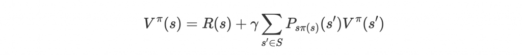
這樣的形式表示 value 是當下 reward R(s) 和所有進入 next state https://chart.googleapis.com/chart?cht=tx&chl=s' 的機率 https://chart.googleapis.com/chart?cht=tx&chl=P_%7Bs%5Cpi(s)%7D(s') 乘上到達 next state 後的 discounted value https://chart.googleapis.com/chart?cht=tx&chl=%5Cgamma%20V%5E%7B%5Cpi%7D(s') 的總和。別忘了後面不過是期望值的計算方法。

畫了一個簡易圖,可以想像因為遞迴關係,我們會先從最後一個 timestep 計算 value(最後一步的 value 就是當下的 reward),一步步往前加總,直到遞迴到 timestep t 時,未來的 t+1 所有狀態都已經有了 value。Discount 以後加上現在獲得的 reward R(s),即可取得這個 state 的 value https://chart.googleapis.com/chart?cht=tx&chl=V%5E%7B%5Cpi%7D(s)

value function
—— Value function as Bellman equation。

這樣的遞迴關係,方便我們用一個 model approximate https://chart.googleapis.com/chart?cht=tx&chl=V%5E%7B%5Cpi%7D,訓練時就用同一個 model 預測 https://chart.googleapis.com/chart?cht=tx&chl=V%5E%7B%5Cpi%7D(s)https://chart.googleapis.com/chart?cht=tx&chl=V%5E%7B%5Cpi%7D(s') 的值,並慢慢調整 model 讓 https://chart.googleapis.com/chart?cht=tx&chl=V%5E%7B%5Cpi%7D 越來越 optimal、Bellman equation 能夠成立。

State-Action Value Function

第二種 value function 稱為 Q-value function,計算在 state s 時,選擇 action a 後,再根據 policy https://chart.googleapis.com/chart?cht=tx&chl=%5Cpi 走的話能獲得的 total expected reward,同樣也能寫成 Bellman equation:
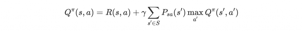
https://ithelp.ithome.com.tw/upload/images/20201009/201306872Q8MaODL8y.png

注意到這個式子和 https://chart.googleapis.com/chart?cht=tx&chl=V%5E%7B%5Cpi%7D(s) 其實是同樣的意思,因為 https://chart.googleapis.com/chart?cht=tx&chl=V%5E%7B%5Cpi%7D(s')%20%3D%20%5Cmax_%7Ba'%7D%20Q%5E%7B%5Cpi%7D(s'%2C%20a')

差異

https://chart.googleapis.com/chart?cht=tx&chl=V%5E%7B%5Cpi%7D(s)https://chart.googleapis.com/chart?cht=tx&chl=Q%5E%7B%5Cpi%7D(s%2C%20a) 看起來頗像,但 Q-value 會更適合用找出最佳 policy。為什麼呢?

首先看到如果訓練出 optimal value function https://chart.googleapis.com/chart?cht=tx&chl=V%5E*(s),最佳 policy 會是:

https://ithelp.ithome.com.tw/upload/images/20201009/20130687eoJkg1iObl.png

而訓練出 optimal Q-value function https://chart.googleapis.com/chart?cht=tx&chl=Q%5E*(s%2C%20a),最佳 policy 會是:

https://ithelp.ithome.com.tw/upload/images/20201009/20130687BudOjEIx2o.png

訓練 Q(s, a) 的話,policy 等於挑最大 Q-value 的 action 就好。但訓練 V(s),卻沒辦法很方便地轉換成我們要的 action,因為還需要 state transition probability。

Q-Learning

從上面我們知道,要找出 policy,首先要先 approximate Q-value function。但是根據上面的數學,似乎需要知道環境的 state transition probability https://chart.googleapis.com/chart?cht=tx&chl=P_%7Bsa%7D 才能計算 Q-value 並訓練 Q-value function。

這次來介紹簡單一點的訓練方法 Q-learning,不用 https://chart.googleapis.com/chart?cht=tx&chl=P_%7Bsa%7D 即可訓練,這種方法稱為 model-free learning。

這裡的 model 是指環境 model,不是 machine learning model。

Q-learning 大致流程如下:

  1. 定義 model 來 approximate Q-value function,可以是簡單的 lookup table,當然還可以是我們最會的 neural network。Model input 會是 state s,output 會是 https://chart.googleapis.com/chart?cht=tx&chl=%7CA%7C 個 Q-value Q(s, a),A 為 action space,包含所有可能動作。
  2. 訓練前隨機 initialize model parameters。同時 intialize 所處環境,從 https://chart.googleapis.com/chart?cht=tx&chl=s_0 開始。
  3. 開始跟環境互動。Model 預測 https://chart.googleapis.com/chart?cht=tx&chl=%7CA%7C 個 Q-value,選擇最大 Q-value 的 action https://chart.googleapis.com/chart?cht=tx&chl=a_0。做出 action 後,環境 transition 到 https://chart.googleapis.com/chart?cht=tx&chl=s_1,並收穫 reward https://chart.googleapis.com/chart?cht=tx&chl=R_1
  4. 更新 parametershttps://chart.googleapis.com/chart?cht=tx&chl=Q(s_0%2C%20a_0)%20%3D%20Q(s_0%2C%20a_0)%20%2B%20%5Calpha%20(R_1%20%2B%20%5Cgamma%20%5Cmax_a%20Q(s_1%2C%20a)%20-%20Q(s_0%2C%20a_0))
  5. 重複 3.4. 直到 Q-value function 收斂。

其中最關鍵的是第四步:

https://ithelp.ithome.com.tw/upload/images/20201009/20130687FZbhSLyTCb.png

https://chart.googleapis.com/chart?cht=tx&chl=%5Calpha 是 learning rate。這個方法其實很直覺,https://chart.googleapis.com/chart?cht=tx&chl=R_%7Bt%2B1%7D%20%2B%20%5Cgamma%20%5Cmax_a%20Q(s_%7Bt%2B1%7D%2C%20a) 是下個 state 實際上的 expected reward,但 model 一開始預測的是 https://chart.googleapis.com/chart?cht=tx&chl=Q(s_t%2C%20a_t),因此差距為 https://chart.googleapis.com/chart?cht=tx&chl=R_%7Bt%2B1%7D%20%2B%20%5Cgamma%20%5Cmax_a%20Q(s_%7Bt%2B1%7D%2C%20a)%20-%20Q(s_t%2C%20a_t),update 時把這個差距藉由 https://chart.googleapis.com/chart?cht=tx&chl=%5Calpha 慢慢補上。

說是實際上的 expected reward,但 https://chart.googleapis.com/chart?cht=tx&chl=R_%7Bt%2B1%7D%20%2B%20%5Cgamma%20%5Cmax_a%20Q(s_%7Bt%2B1%7D%2C%20a) 中的 Q 在訓練中也只是估計值,主要是以環境真正返回的 https://chart.googleapis.com/chart?cht=tx&chl=R_%7Bt%2B1%7D 為目標邁進。

Deep Atari

(Mnih et al., 2013) Playing Atari with Deep Reinforcement Learning
(Mnih et al., 2015) Human-level control through deep reinforcement learning

介紹完 RL 的原理和 Q-learning 的學習方法,我們再藉由經典的 Atari paper 稍微統整一下剛剛的知識,還有 deep learning 如何和 Q-learning 結合。

Problem

Atari 是一套經典的電玩機遊戲,裡面包含的遊戲大多只需要簡單幾個控制:

games
—— Atari 遊戲畫面。

這篇 paper 主要目的是用 deep learning 結合 reinforcement learning 訓練這套遊戲的 AI。這在當時(2013 年)是一項創舉,開了 DL 結合 RL 的先河。

RL 架構

首先是 RL 框架的定義:

  • Agent:Atari AI。
  • Environment:Atari 模擬器。
  • State:遊戲畫面。
  • Action:控制動作,上下左右等等。
  • Reward:動作後遊戲分數的改變。

這可以說是 RL 最簡單的設定:現有的模擬器、簡單的控制動作、容易定義的 reward。新手想玩 RL 可以先從這類的任務下手。

訓練方法:Deep Q-Network (DQN)

Deep Q-network (DQN) 是 Q-learning 的一種,其中 Q-value function 用 neural network 來 approximate。

Model 是個簡單的 CNN model。Input 遊戲畫面作為 state s,經由 CNN 提取特徵,預測 https://chart.googleapis.com/chart?cht=tx&chl=%7CA%7C 個 Q(s, a)。Policy 會選擇使 Q(s, a) 最大的 a 當作控制動作。動作後由遊戲模擬器返回分數作為 reward,藉由 Q-learning update rule 更新 model 參數。

DQN
—— DQN model。

比較值得一提的是一些訓練技巧:

  • https://chart.googleapis.com/chart?cht=tx&chl=%5Cepsilon-greedy:一種平衡 exploration 和 exploitation 的技巧。當 agent 在玩遊戲時,保守一點可能會永遠選擇 Q-value 最大的 action 來穩穩獲得 reward,這個稱為 exploitation。但是太保守的話,他可能會錯失一些可以帶來極大 reward 的動作,因為他從來都不敢嘗試,也就不知道這些動作值得做。Exploration 就是讓 agent 能跳脫現有的 policy,不根據 Q-value 隨機選擇下個動作。在訓練時需要平衡兩者,而 https://chart.googleapis.com/chart?cht=tx&chl=%5Cepsilon 是介於 0 到 1 的值,定義跳脫 Q-value 隨機選擇動作的機率。
  • Experience replay:把所有跟環境互動的經驗記在一個 buffer 裡面,訓練時從 buffer 隨機抽取經驗學習。這樣做可以有效重複利用以前的經驗進行訓練,同時打散不必要的時間關係。
  • Target network:在 Q-learning 中,每一次 Q 的 update 都包含了下一步過後的 Q-value https://chart.googleapis.com/chart?cht=tx&chl=Q'。但如果 Q 和 https://chart.googleapis.com/chart?cht=tx&chl=Q' 都是從同一個 model 預測的話,那麼等於更新完 model 之後,剛剛的 https://chart.googleapis.com/chart?cht=tx&chl=Q' 同時失效了。這樣會造成訓練不穩定,有點像一隻狗頭追著尾巴跑。所以 paper 中用了兩個 network,一個訓練用,另一個是 target network,每隔一段時間從訓練用的 network 複製過來,接著靜置一段時間,讓這段期間的 update 更穩定一點。

Results

簡單秀一下 value function 的 visualization:

value function
—— Game Breakout value function visualization。

上圖 Breakout 遊戲,左右控制下方的板子,讓球反彈打碎上方的方塊。y 軸 V 代表每個 state 的 total expected reward。右方 4 球彈到最上面後,可以預期會在上面反彈一陣子,能獲得很高的分數。

Q-value function
—— Game Pong Q-value function visualization。

上圖 Pong 遊戲,上下控制左右方塊,將球反彈到對面。y 軸 Q 代表每個 state 之下進行 action No-Op、Up、和 Down 的 total expected reward。中間 2、3 顯示右邊的方塊應該要往上走,才能接到球反彈到對面。

結語

RL 的框架很彈性,可以套用在很多任務上進行訓練。但就算是 Atari 這麼基本的 task 都還需要很多額外的訓練技巧才能成功訓練,所以其實 RL 最困難的就是訓練的穩定性,還有訓練不成功時怎麼找出改進方法。

這次篇幅有點緊湊,一把從 RL 原理、value function、Q-learning,帶到 DQN 的 paper,內容偏學術一點。下一篇會藉由實作經典的 CartPole 問題帶大家更實際理解 RL。

Checkpoint

  • Reinforcement learning 和 supervised / unsupervised learning 比,最大的差異在於從何學習。請問兩者的學習來源分別為何?
  • 能否畫出 reinforcement learning 中 agent 和 environment 的互動過程?
  • Discount factor https://chart.googleapis.com/chart?cht=tx&chl=%5Cgamma 用途為何?
  • Policy 簡單來說是什麼?
  • Value function 和 Q-value function 主要是在計算什麼?
  • Q-learning 中的 model,input 和 output 為何?Agent 會怎麼選擇下一步 action?
  • DQN 中的 neural network 主要負責做什麼?
  • 請解釋何謂 exploitation v.s. exploration。
  • 請看一下 Q-learning 的 update rule。在 DQN 中使用 target network,是為了穩定 update rule 中的哪一項?

參考資料

  1. ? CS229 Lecture Notes: Reinforcement Learning and Control
  2. CS230 Lecture Slides: Deep Reinforcement Learning
  3. CS231n Lecture Slides: Reinforcement Learning
  4. MIT 6.S091 Lecture Slides: Introduction to Deep Reinforcement Learning
  5. CS234 Lecture Slides: Tabular RL policy evaluation
  6. CS234 Lecture Slides: Q-learning
  7. MIT 6.S191 Lecture Slides: Deep Reinforcement Learning
  8. (Arulkumaran et al., 2017) A Brief Survey of Deep Reinforcement Learning

上一篇
Day 23 / DL x CV / CV 總結與發展
下一篇
Day 25 / DL x RL / Hello Reinforcement Learning —— CartPole
系列文
Knock Knock! Deep Learning31
圖片
  直播研討會
圖片
{{ item.channelVendor }} {{ item.webinarstarted }} |
{{ formatDate(item.duration) }}
直播中

尚未有邦友留言

立即登入留言