回顧一下昨天提到的，我們希望透過將 attention 機制加到 LSTM 中藉此找出每段語音中重要的
部份。因此原本的 LSTM 架構就會修改成圖 1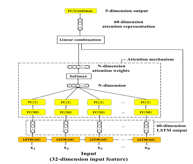

圖1: LSTM with attention mechanism動態模型架構圖

LSTM 由原本的兩層改為一層(60 個神經元、activation function 為 tanh、ReLU)，attention 的輸入為LSTM 每一個時間點的輸出 ，接下來使用兩層的全連接層(FC, 第一層 50 個神經元，activation function 為 tanh、ReLU；第二層 1 個神經元，沒有 activation function)，第二層的輸出以 softmax 轉換成機率的形式，產生的向量即為每一個時間點 attention weights 。將 與前面 LSTM 每一個時間點的輸出 相乘並將相乘結果加總，以 attention representation z 表示。Attention weights 與 LSTM 的輸出相乘的結果即可解釋為每一個時間點對於整段話語的貢獻值。最後將 attention representation 傳遞至輸出層。

其中 T 為輸入序列中最大的時間點值而 、 為 attention 機制中兩層全連接層的權重矩陣。

加入 attention module 後的模型程式如下：

dynamic_input = Input(shape=[max_length, args.dynamic_features], dtype='float32', name='dynamic_input')

lstm1 = LSTM(60, activation='tanh', return_sequences=True, recurrent_dropout=0.5, name='lstm1')(dynamic_input)
#attention mechanism module
attention_dense1 = Dense(args.attention_layer_units, activation='tanh', use_bias=False, name='attention_dense1')(lstm1)
attention_dense2 = Dense(1, use_bias=False, name='attention_dense2')(attention_dense1)
attention_flatten = Flatten()(attention_dense2)
attention_softmax = Activation('softmax', name='attention_weights')(attention_flatten)
attention_multiply = multiply([lstm1, attention_permute])
attention_representation = Lambda(lambda xin: K.sum(xin, axis=1), name='attention_representation')(attention_multiply)# 60

# classifier module
output = Dense(args.classes, activation='softmax', name='output')(attention_representation)
model = Model(inputs=dynamic_input, outputs=output)
model.summary()

分類結果如表 1。
Model | UA recall (tanh) | UA recall (ReLU)
------------- | -------------
LSTM with attention | 47.2% | 20.0%
表1: LSTM with attention 分類結果

加入 attention 後 UA recall 可以達到 47.2%，與 basic LSTM 相比有明顯的提升。 另外，從 basic LSTM 與 LSTM with attention 中我們發現在動態模型中以 ReLU 為 activation function 的話 UA recall會很差只有 20.0%，原因應為使用 ReLU 為 activation function 的話，特徵值中所有負數的部份都會變為 0，使得 LSTM 會有多個時間點的輸出皆為0，導致模型無法分類出此輸入屬於何種類別。
LSTM with attention 分類結果的混淆矩陣如下
/ | A | E | N | P | R | UA recall
------------- | -------------
A | 375 | 119 | 54 | 35 | 28 | 61.4%
E | 286 | 815 | 251 | 31 | 125 | 54.0%
N | 821 | 979 | 2,309 | 718 | 550 | 42.9%
P | 9 | 6 | 54 | 130 | 16 | 60.5%
R | 117 | 76 | 132 | 128 | 93 | 17.0%
Avg.recall | - | - | - | - | - | 47.2%
表2: LSTM with attention 分類結果混淆矩陣

為了更進一步探討 attention 機制的影響，我們將 attention weights 標準化至相同的時間範圍(max_slot=100)後所得到分佈圖如圖 2 (a), (b)。從圖中我們可以觀察到，平均而言，話語中間的部份通常比兩邊邊緣的部份有著更大的 attention weights。這說明了情感表達通常都集中在語音中間的區段。
昨天的內容中有提到說為了讓每一筆輸入語音檔長度相同我們會做 padding 補 0 的動作，因此在將 attention weights 視覺化的過程中需要將額外補 0 的部分排除 (delete_padding_part())

# attention_visualize.py
def delete_padding_part(data, seq_length):
    no_padding_data = []
	  for i in range(data.shape[0]):
		    no_padding_start_pos = 2453 - seq_length[i]
		    temp = data[i][no_padding_start_pos:]
		    no_padding_data.append(temp)
	no_padding_data = np.asarray(no_padding_data)
	return no_padding_data

def avg_distribution(data, max_slot=100):
    seq_slot_value = []
	  for i in range(data.shape[0]):# each sequence
		    interval = len(data[i])/max_slot
		    temp = []
		    slot_count = 0
		    j = 0.0
		    while slot_count < max_slot:# each slot
			      slot_sum = np.zeros(60)
			      count = 0
			      if math.floor(j) != math.floor(j+interval):
				        for k in range(math.floor(j), math.floor(j+interval)):
					          if k >= len(data[i]):
						            break
					          count += 1
					          slot_sum += data[i][k]
			      else:
				        slot_sum = np.zeros(60)
			      temp.append(slot_sum)
			      slot_count += 1
			      j += interval
		    seq_slot_value.append(temp)
	  seq_slot_value = np.asarray(seq_slot_value)
	  # calculate the average by each column
	  seq_slot_avg = []
	  for i in range(seq_slot_value.shape[1]):
		    col_sum = np.sum(seq_slot_value[:, i], axis=0)
		    col_sum_avg = col_sum / (seq_slot_value.shape[0])
		    seq_slot_avg.append(col_sum_avg)
	  seq_slot_avg = np.asarray(seq_slot_avg)
	  return seq_slot_avg

最後，從圖 2 (c), (d) 的各類別 t-SNE 分佈圖中我們可以看出，不同類別資料的分佈情形明顯的重疊一起。
可透過 sklearn.manifold.TSNE 來實作

from sklearn.manifold import TSNE

def tsne(X, n_components):
    model = TSNE(n_components=2, perplexity=40)
    return model.fit_transform(X)

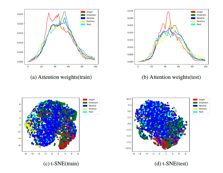
圖 2: 訓練集與測試集各類別 attention weights、t-SNE 分佈圖。紅色：angry，綠
色：emphatic，藍色：neutral，黃色：positive，青色：rest

介紹完了靜態模型跟動態模型，明天我們將會使用藉由不同模型間的結合來提高模型效能的方法 - 集成學習 (ensemble learning)。