零、前言

在上一篇中，我們透過實際計算 Loss Function 並執行梯度下降法時，發現設定學習率會直接影響到機器訓練時的表現，對此我們可以透過更改學習率進行調整。那這也是屬於比較單純的函數。但我們從大一的微積分中，也有學過些具有 Local Minima 或 Saddle Point 的函數，這些如果發生在機器學習的 Loss Function 上，又會發生甚麼狀況呢？

一、最小值的情況

[0]

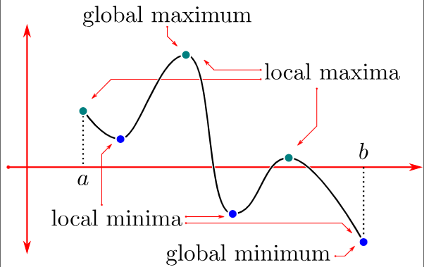
我們先回到數學上看來看，一個函數可能會有區域極值與全域極值，而在梯度下降法中，我們的目的是找出損失函數的最小值，所以目標會放在最小值相關的部分。相關定義如下：

Let D be the domain of the function and :

1. is called the Absolute Minimum Value if and .

2. is called the Local (eg. Relative) Minimum Value if there’s an open interval , which contains , such that .

假設有一個函數是 ，在學習率為 0.15 的情況下會收斂到 Local Minimum：

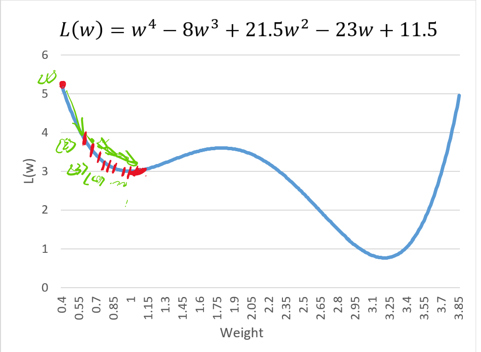
從以上情況的角度來在分析 Loss Function 的時候，我們不會希望在調整權重時，發現自己分析到的一直都不是最佳解，這樣不是我們樂見的。那在做梯度下降法的分析過程中，我們也要避免學習率的步伐率領我們走入 Local Minimum 而非 Global Minimum 的情況。

二、多變數的 Loss Function

針對這次的章節，我重新設計了一個本身具有這些特性的函數

我們逐一來分析：首先為了讓分析稍微簡單些，我們先將 設定為 1 以便進行分析，並計算其梯度：

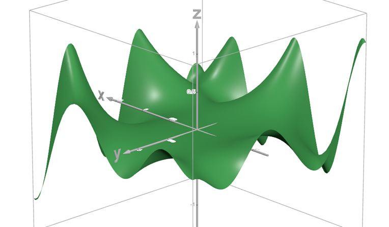
針對這情況，我們可以畫出函數圖形：

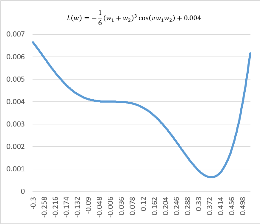
這個Loss Function 的函數中，如果我們將起始點 設定為 0.3，學習率 設定為 22，這時 會迭代出以下結果：

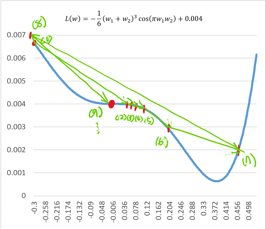
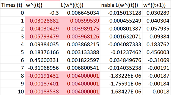
我們會發現這個紅點代表 Loss Function 已經收斂了，但是這個值好像並不是最佳的情況。那這個點又是甚麼呢？

1. Inflection Point

我們可以看出來這圖形的權重值在接近 0（紅點）的時候，函數的曲面特性發生轉折，也就是說在紅點左側可以看出是上凹的特性，紅點的右側屬於下凹，這個點在平面座標的曲線上，我們稱做「轉折點」，其定義上為：

A point P on the graph of a function y=f\left(x\right) is identified as an Inflection Point when the function is continuous at that point, and the curvature of the graph transitions from concave upward to concave downward at P, and conversely.

但是我們在機器學習中，並不會把這個點稱為 Inflection Point。這是為何呢？

我們回來看以下方程式

在做機器學習分析的時候，模型不會只有一個權重值，而一個 weight 只能顯示出 Loss Function 在一個方向的變化，而無法反映出在分析考量其他的 weight 之後對於 Loss Function 變化的影響，所以我們勢必要用立體座標來看出他們之間的關係。

而對於立體座標來說，Loss Function 便不是一個平滑的曲面，而是充滿很多的凹凸點，所以要成為 Inflection Point，從定義上看就必須讓 x 軸（）與 y 軸（）上的曲率（二次導數）都發生改變才行，這是很難以滿足的條件。

2. Saddle Point

而在立體座標圖中，還有一個點稱為「鞍點」，其定義如下：

A saddle point, also known as a minimax point, refers to a point situated on the surface of a function's graph. At this point, the derivatives along orthogonal directions are all zero, marking it as a critical point. However, it does not qualify as a local extremum of the function.[2]

實務分析上，大部分的 Loss Function 在進行梯度下降法的分析時，基本上都是掉入像是 Saddle Point 的轉折點，所以我們只需要透過一些技巧，避免掉入或是可以跳出 Saddle Point，就可以擺脫無法得到最佳解的情況，而並非僅限於 Inflection Point。這些也是為何我們在做梯度下降法時，為何會偏好稱 Saddle Points 的原因。
而脫離 Saddle Points 最常用的方式包含 Momentum 、學習率衰減、隨機梯度下降等方法。

[3]

而對於多變數函數，最適合找出 Saddle Point 的方式就是利用 Hessian 矩陣，但這計算就更為複雜了，所以我就算完之後簡單附上。

3. 使用 Hessian Matrix 找出鞍點

Hessian Matrix 定義可以參考這邊：https://en.wikipedia.org/wiki/Hessian_matrix#:~:text=In%20mathematics%2C%20the%20Hessian%20matrix,a%20function%20of%20many%20variables.

簡單來說，如果你從否些角度來看鞍點就像山頂，但在否些角度上看起來像在山谷。而在這些點上透過 Hessian Matrix 計算出來特徵值包含正定與負定矩陣，那這個點就會是鞍點（可以參考線性代數）。對於方程式：

我們引用 Hessian Matrix 寫出：

我們首先要先分別解出其梯度值（一次偏微分）

二次偏微分 \nabla^2L：

接下來基本上就是透過一些數學軟體來處理了～

三、結語

以上大約是我們在進行 SGD 會遇到的狀況，並且為其做一個案例示範。這內容也包含我在學習這部分時，所想到的一些問題，並且透過數學方式解決的過程。而我們知道基本的最佳化模型以及其訓練過程之後，我們就可以去了解其他種類的 Loss Function 與 Optimizer 可以幫助我們解決甚麼樣的問題了！

四、參考資料

[0] Local and Global Maxima and Minima：https://personal.math.ubc.ca/~CLP/CLP1/clp_1_dc/ssec_maxmin.html
[1] Inflection Point 與 Saddle Point：https://math.stackexchange.com/questions/2446431/whats-the-difference-between-saddle-and-inflection-point
[2] Saddle Point Definition：https://en.wikipedia.org/wiki/Saddle_point#:~:text=In%20mathematics%2C%20a%20saddle%20point,local%20extremum%20of%20the%20function
[3] Animation of dynamics of Various Optimizer：https://cs231n.github.io/neural-networks-3/