tl;dr

• 我們今天會實際驗證兩個 embed model(text-embedding-3-small 和 text-embedding-ada-002) 在我們資料集上的表現
• 它們的任務是比較 ground-truth 以及 llm-prediction 的相似性，使用的是 SemanticSimilarityEvaluator
• 因為我們是在比較 evaluator 的效果，所以這次的實驗本質上是 Evaluating Evaluator
• 數據上兩者的 precision 和 recall 分別為：

  # small-3 result: 
  {'precision': 0.9032258064516129, 'recall': 0.9655172413793104}
  # ada result: 
  {'precision': 0.9333333333333333, 'recall': 0.9655172413793104}
  

  • 可以看到在相同 recall 下，ada-002 的 precision 還略高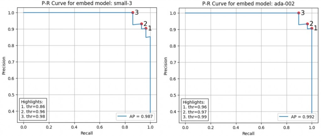
• 我們繪製了兩者的 P-R Curve
  • 
• 完整的程式碼在 這裡

我們接下來就來看看這是怎麼做的吧

Action

1. 首先是分別把兩者的 similarity score 跑出來

• 在專案路徑下執行: python semantic_similarity.py
  • 若對於什麼是 SemanticSimilarityEvaluator 不熟悉，可以參考我們在 day19 的介紹
• 我們的 output 會是一個 嵌套的 dictionary
  • 首先可以直接用 qid 來獲取每筆資料的內容
  • 針對每筆資料，主要有 keys:
    • reference_answer(str): 原始任務的 ground-truth
    • response(str): llm 針對原始任務的 response
    • semantic_score(float): embedding model 計算出針對兩者的相似值
      • 越高越像
  • 點我看結果: semantic_similarity result
• 此外我們還要獲取我們在 day20 用 exact_match 跑出來的兩者相似性的結果
  • 他主要的 key 是 ispass，指出 reference_answer 與 response 是否 match
    • 其他包含 qid, label, pred 用來協助我們觀察不 match 的情況是發生了什麼事
  • 點我看結果: normalized_exact_match_result

2. 直接用 plot 比較

• 這張圖的 x 軸 是原是資料的 id ，所以每個 x 軸代表了某一筆資料
• y 軸是 reference_answer 與 llm_prediction 的 similarity score
• 綠點是 exact match 的結果，因為只有通過跟不通過，所以我們設置通過相似度為1，不通過相似度為0
• 橘色虛線是 text-embedding-ada-002 跑出來的結果
• 藍色虛線是 text-embedding-3-small 跑出來的結果

觀察

• 首先是我們發現 ada002 在 score 的 range 比較窄
  • 也就是說在 embedding 空間上 small-3 其實把資料分的比較開
• 第二是乍看之下在 Exact Match pass 的 case (綠點 y 座標為 1)的部分， embedding 大部分都有給到很高的相似性

3. 我們來直接基於兩個 threshold 看 precision 跟 recall

• 這邊我們試用看看 huggingface 的 evaluate

  import evaluate  # pip install evaluate
  
  def _get_binary_prediction(pred, thr):
      return [0.0 if p <= thr else 1. for p in pred]
  
  def _get_precision_recall(pred, label):
      precision_metric = evaluate.load("precision")
      recall_metric = evaluate.load("recall")
  
      combined = evaluate.combine([precision_metric, recall_metric])
      results = combined.compute(predictions=pred, references=label)
      return results  # dict 
  
  def get_precision_recall(pred, label, thr):
      binary_pred = _get_binary_prediction(pred, thr)
      result = _get_precision_recall(binary_pred, label)
      return result  # dict 
  
  

• 在 threshold = 0.8557835443653601 下:

  # small-3 result: 
  {'precision': 0.9032258064516129, 'recall': 0.9655172413793104}
  # ada result: 
  {'precision': 0.7631578947368421, 'recall': 1.0}
  

  • 這邊 small-3 的結果可能稍好一點
  • 雖然 ada 的 recall 有到 1.0，但 precision 只有 .76 以我們要做 evaluation 的任務來說 誤報太嚴重

• 在 threshold = 0.9676289405210952

  # small-3 result: 
  {'precision': 0.9285714285714286, 'recall': 0.896551724137931}
  # ada result: 
  {'precision': 0.9333333333333333, 'recall': 0.9655172413793104}
  

  • 這次情況反轉了，ada002 比較好，他給出了比較好的 precision 與 recall
  • 而 small-3 漏掉了 1 成的錯誤

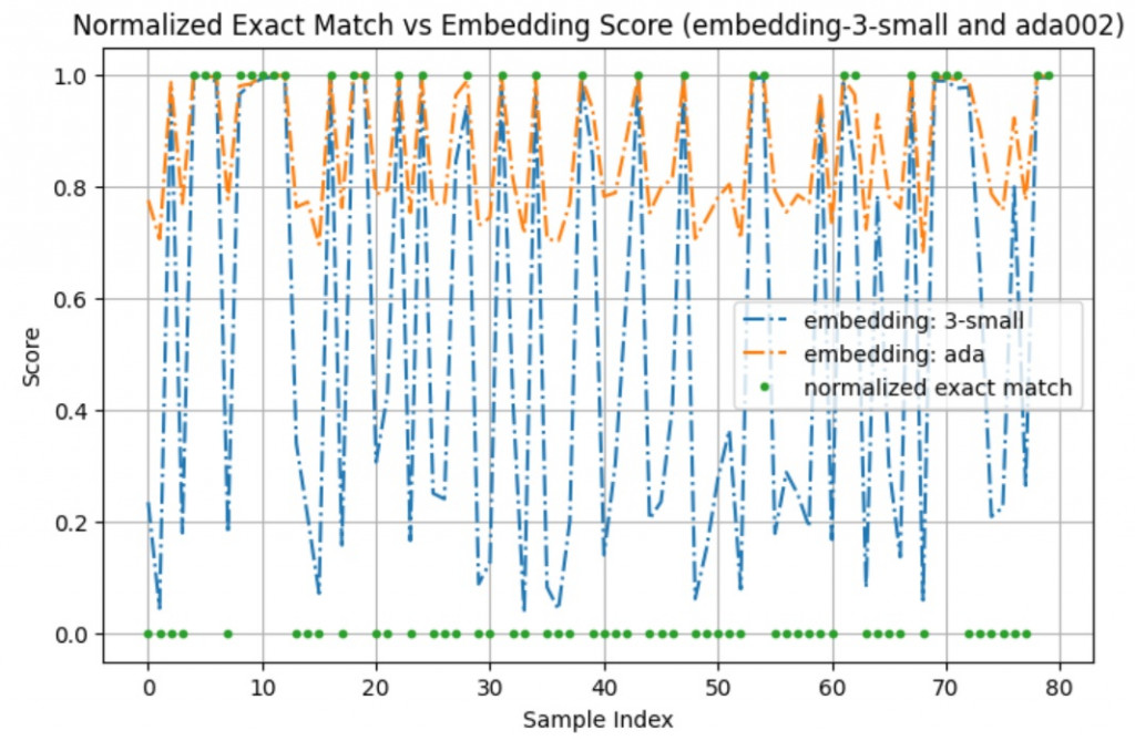
• 這邊其實呼應了我們前面的觀測，ada002 的 similarity score 在我們的任務上看起來分布比較窄

• 所以其實像這種只有 similarity score 的任務，我們需要給每個 model 不同的 threshold

• 那問題就來了，這邊的這兩個 threshold 是怎麼得到的？

4. 這兩個 threshold 怎麼來的?

4.1 先得到所有的 precision, recall 與 threshold

• 我們可以基於 PR-Curve 來選擇

  • 首先把我們的 similarity score 排序
  • 接著我們把每個 similarity score 當作 threshold
  • 這樣我們就可以分別計算 precision 和 recall
  • 最後我們會分別插入 precision = 1, recall = 0 的起始點
    • 所以我們的 precision 與 recall 分別有 num_data +1 個
    • 我們的 threshold 有 num_data 個

• 我們這邊直接基於 sklearn 的 precision_recall_curve 來得到 precision, recall 與 threshold

  • 它的實作就是我們上面的描述

• 此外我們順勢把 ap 也算出來， ap 表示的就是 precision_recall_curve 的曲線下面積

  import numpy as np
  from sklearn.metrics import precision_recall_curve
  from sklearn.metrics import average_precision_score
  
  precisions, recalls, thresholds = precision_recall_curve(labels, ada_scores)
  print(type(precisions), precisions.shape, type(recalls), recalls.shape, type(thresholds), thresholds.shape)
  ap = average_precision_score(labels, ada_scores)
  

  • 怎麼實作這個 ap 的計算在 notebook 的 average_precision_from_pr 函數

4.2 計算 f1_score 與 挑出 topk 個 f1_score

• f1 score 是一 precision/recall 的調和平均，目的是協助我們找到一個 precision 與 recall 的權衡，可以參考 sklearn-f1_score
• 我們這邊挑出最高的 k 個 f1 score ，並且把資料存出來成為我們的 highlight

  def get_f1_score(precisions, recalls):
      # from precision and recall
      f1_scores = np.where(
          (precisions + recalls) > 0,
          2 * precisions * recalls / (precisions + recalls),
          0.0,
      )
      return f1_scores
  def get_topk_highlight(precisions, recalls, k=3):
      f1_scores = get_f1_score(precisions, recalls)
      topk_idx = np.argsort(-f1_scores)[:k]
  
      highlights = []
      for idx in topk_idx:
          thr = None if idx == 0 else thresholds[idx - 1]
          highlights.append({
              "f1": float(f1_scores[idx]),
              "precision": float(precisions[idx]),
              "recall": float(recalls[idx]),
              "threshold": None if thr is None else float(thr),
              "idx": int(idx),
          })
      return highlights
  

• ada002 的 highlight 在 top 3 的結果為：

  [{'f1': 0.9508196721311475,
    'precision': 0.90625,
    'recall': 1.0,
    'threshold': 0.9642988120688676,
    'idx': 48},
   {'f1': 0.9491525423728815,
    'precision': 0.9333333333333333,
    'recall': 0.9655172413793104,
    'threshold': 0.9676289405210952,
    'idx': 50},
   {'f1': 0.9454545454545454,
    'precision': 1.0,
    'recall': 0.896551724137931,
    'threshold': 0.9899387683709545,
    'idx': 54}]
  

5. 繪圖

```
import matplotlib.pyplot as plt
from matplotlib.offsetbox import AnchoredText

plt.figure(figsize=(6, 5))
plt.plot(recalls, precisions, label=f"AP = {ap:.3f}")

# highlight 點只標號碼
for i, h in enumerate(highlights, 1):
    plt.scatter(h["recall"], h["precision"],
                s=20, facecolors="none", edgecolors="red", linewidths=2)
    plt.text(h["recall"], h["precision"], f"    {i}",
             fontsize=15, ha="center", va="center", color="black")

# thresholds 說明，放左下角
thr_lines = [f"{i}. thr={h['threshold']:.2f}" for i, h in enumerate(highlights, 1)]
txt = "Highlights:\n" + "\n".join(thr_lines)
at = AnchoredText(txt, prop=dict(size=10), frameon=True, loc="lower left")
at.patch.set_alpha(0.8)
plt.gca().add_artist(at)

plt.xlabel("Recall")
plt.ylabel("Precision")
plt.title(f"P-R Curve for embed model: {model_base_name}")
plt.legend(loc="lower right", framealpha=0.9)  # 這裡只放 AP
plt.grid(True)
plt.show()
```

• 這就是最一開始上的圖了
  • 我們這邊除了繪製 P-R Curve 以外
  • 我們在圖上把 top-3 的 f1 score 點標示出來
    • 可以有一個直觀的理解就是 f1 score 高的點就會發生在 P-R Curve 靠近右上角的角點
  • 由於每個 precision 與 recall 同時對應了某個 threshold，因此我們可以取出我們要的 threshold

Summary:

• 我們今天的首要目標是驗證兩個 embedding model (text-embedding-3-small、ada-002) 作為 evaluator 的表現

• 數值上來說最好的結果是:

  • {'precision': 0.9333333333333333, 'recall': 0.9655172413793104}

• 這刷新了兩層我們的認知：

  • 原來 0.93 的 precision 其實沒有我們想像中的高
    • 總感覺我們很容易找到 embedding model 不 work 的點
  • 原來 embedding model 也沒有我們本來想像中的那麼不准
    • 刻板印象上覺得這個應該不太 work

• 在這中間我們遇到了 threshold 要怎麼選的問題

  • 我們實際走訪一次用 P-R Curve 來協助我們決定 threshold 的流程
  • 針對 F1 Score 我們今天刷新了一個它的直觀理解
    • 原來 P-R Curve 的角點其實就是 F1 Score 的 Top-k

• 我們實際比較了 新版本的 embedding-small-3 與 舊版的 ada-002

  • 最一開始的 plot 會讓我們以為 ada-002 似乎是比較差的結果
  • 但實際選完 threshold 之後結論反轉了，它在我們的這個任務上其實是比較好的選擇

• 今天介紹的方法最大的缺點在於: 一定要先有 ground-truth 這些計算才能成立

  • 要解決這個問題，一個明顯的方法是我們可以先選出一小批多樣的資料
  • 接著進行一次人工標註，來取得一部分帶有 ground-truth 的資料
  • 我們預計後續會介紹 label-studio 的使用，一個用來協助創建資料收集介面的工具