筆者在作上一篇時卡住很久,因為,碰到很多術語,搞得頭暈腦脹,因此本篇花點時間將心得整理起來,與同好共享。
內容大致如下:
成效衡量指標(Metrics)通常分三種 -- 準確率(Accuracy)、精確率(Precision)、召回率(Recall)。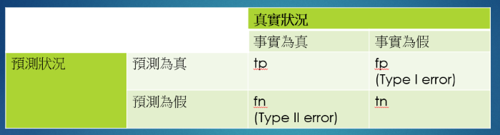
圖. 成效衡量指標(Metrics)的四種情況
NLTK提供相關的函數,可以計算上述指標,用下列一段程式說明,就會很清楚。
from __future__ import print_function
from nltk.metrics import *
training='雞 貓 雞 貓 狗 人'.split()
testing ='雞 貓 雞 貓 貓 貓'.split()
# 6個猜對4個
print("accuracy=", accuracy(training,testing))
trainset=set(training)
testset=set(testing)
print("trainset=", trainset)
print("testset=", testset)
# 猜的全部在4"種"類別內
print("precision=", precision(trainset,testset))
# 4"種"猜對兩種
print("recall=", recall(trainset,testset))
通過上述的範例說明,我們可以根據解決問題的目標來選擇成效衡量指標。
本例來自這裡,假設有兩個文件:
(1) John likes to watch movies. Mary likes movies too.
(2) John also likes to watch football games.
綜合兩個文件,共有10個單字如下:
[
"John",
"likes",
"to",
"watch",
"movies",
"Mary",
"too",
"also",
"football",
"games"
]
兩個文件的詞袋(Bag Of Words)如下:
(1) [1, 2, 1, 1, 2, 1, 1, 0, 0, 0]
(2) [1, 1, 1, 1, 0, 0, 0, 1, 1, 1]
粗體的2代表第一個文件出現兩個 likes,但並不記載 likes 的位置,這種只記次數,不記位置是詞袋(Bag Of Words)的特色。
Continuous Bag-of Words(CBOW):是將一段句子的中間字當作label,其左右文字為input words,所以是多個字input 一個輸出label。
[
"John to", ==> likes
"likes watch", ==> to
"to movies", ==> watch
"movies likes", ==> Mary
"Mary movies", ==> likes
"likes movies", ==> movies
]
n元語法又分一元(unigram)、兩元(bigram)、三元(trigram)、四元(quadgram)、...等語法,就是記錄前面幾個單字,例如兩元語法(bigram)就是記錄前兩個單字,以上述第一句為例,就等於:
[
"John likes",
"likes to",
"to watch",
"watch movies",
"Mary likes",
"likes movies",
"movies too",
]
另外衍生出 k-skip-n-gram,例如 1-skip-2-grams,就等於:
[
"John to",
"likes watch",
"to movies",
"movies likes",
"Mary movies",
"likes movies",
"movies too",
]
每次跳一個單字,取兩個單字,即一次只輸入一個字,輸出的label 為其前後一定距離內的文字。
Google 創造的 Word2Vec 詞向量模型就是利用 CBOW 及 skip-gram 計算詞向量。
句子通常包含關鍵單字,透過關鍵字,我們可以瞭解整個句子的大意,tf-idf 主要是希望單字的重要性隨著它在文件檔案中出現的次數成正比增加,即term frequency,但要降低一些語助詞、介係詞、代名詞的重要性,會再定義一個指標,隨著它在語料庫中出現的頻率成反比下降,即inverse document frequency。所以,『詞頻』(term frequency,tf)是單字在文件中出現的次數,『逆向檔案頻率』(inverse document frequency,idf)是『所有文件數』除以『有出現該單字的檔案數』,其中 idf 分母通常會加1,避免除以0的問題,另外為避免極端值影響過大,故取 log,tf-idf公式如下:
tf-idf = tf * idf。
我們來看一個NTLK範例。
import nltk.corpus
from nltk.text import TextCollection

# 載入NLTK的範例文句
from nltk.book import text1, text2, text3
# text1 = "Moby Dick by Herman Melville 1851"
# text2 = "Sense and Sensibility by Jane Austen 1811"
# text3 = "The Book of Genesis"
# ...
# text9 = "The Man Who Was Thursday by G . K . Chesterton 1908"

# 使用 TextCollection class 計算 tf-idf
# input為 text1, text2, text3
mytexts = TextCollection([text1, text2, text3])

# 計算 tf,例如,book在text3的tf
# tf = text.count(term) / len(text)
mytexts.tf("book", text3)
# 2.233937985881512e-05

# 計算 idf,例如,book在text1、text2、text3的idf
# idf = (log(len(self._texts) / matches) if matches else 0.0)
mytexts.idf("Book")
# 1.0986122886681098
NER是一種解析文件並標註各個實體類別的技術,例如人、組織、地點...等。NLTK支援此一功能,包含兩種標註函數ne_chunk及Stanford NER,ne_chunk 程式如下:
from nltk import ne_chunk
from nltk import word_tokenize
sent = "Mark is studying at Stanford University in California"
print(ne_chunk(nltk.pos_tag(word_tokenize(sent)), binary=False))
# output
# (PERSON Mark/NNP)
# is/VBZ
# studying/VBG
# at/IN
# (ORGANIZATION Stanford/NNP University/NNP)
# in/IN
# (GPE California/NNP))
除了詞性(Part Of Speech, POS)外,也標註出 PERSON、ORGANIZATION 等命名實體,有助於文件的解析。NLTK還能解析命名實體間的關係,範例如下:
import re
IN = re.compile(r'.*\bin\b(?!\b.+ing)')
for doc in nltk.corpus.ieer.parsed_docs('NYT_19980315'):
    for rel in nltk.sem.extract_rels('ORG', 'LOC', doc, corpus='ieer', pattern = IN):
        print(nltk.sem.rtuple(rel))
# [ORG: 'WHYY'] 'in' [LOC: 'Philadelphia']
# ...
# 'Bastille Opera'] 'in' [LOC: 'Paris']
# ...
# 'Georgia-Pacific'] 'in' [LOC: 'Atlanta']
針對語言的前置處理,我們就能對文句有較深刻的認識,畢竟,語言不是人類與生俱來的本能,必須透過後天學習而來,因此,模仿人類神經的 Neural Network 演算法也要先了解一些語言的特性,才能正確地分類及預測吧,就像AlphaGo下圍棋,要先輸入圍棋的規則。
下次,我們就繼續討論『自然語言處理』的應用吧。