[第六天] 資料分類 Support Vector Machines (2)

2019鐵人賽 svm

theneo

2018-10-20 23:02:03

23901 瀏覽

分享至

今天就來實際跑一下SVM的套件吧～
參考網站

這邊先說明一下首先定義 make_meshgrid 函數的用意是為了先好一個密密麻麻的網格位置，這些網格只要呈現在現有資料範圍附近（這裡只呈現最大值＋１最小值－１之間的範圍）。將這些密密麻麻的位置套入train好的SVMmodel再根據他得出來的值畫不同顏色。當這些點很密自然就會呈現不同顏色的區塊，再畫上資料點就可以跟model預測範圍結合一起即可以看出哪些資料點被誤判～～

%matplotlib inline

import numpy as np
import matplotlib.pyplot as plt
from sklearn import svm, datasets

def make_meshgrid(x, y, h=.02):
    """Create a mesh of points to plot in
    Parameters
    ----------
    x: data to base x-axis meshgrid on
    y: data to base y-axis meshgrid on
    h: stepsize for meshgrid, optional
    Returns
    -------
    xx, yy : ndarray
    """
    x_min, x_max = x.min() - 1, x.max() + 1
    y_min, y_max = y.min() - 1, y.max() + 1
    xx, yy = np.meshgrid(np.arange(x_min, x_max, h),
                         np.arange(y_min, y_max, h))
    return xx, yy
    
 def plot_contours(ax, clf, xx, yy, **params):
    """Plot the decision boundaries for a classifier.

    Parameters
    ----------
    ax: matplotlib axes object
    clf: a classifier
    xx: meshgrid ndarray
    yy: meshgrid ndarray
    params: dictionary of params to pass to contourf, optional
    """
    Z = clf.predict(np.c_[xx.ravel(), yy.ravel()])   #這些密密麻麻的點都進去model預測類別
    Z = Z.reshape(xx.shape)
    out = ax.contourf(xx, yy, Z, **params)    #就可以把不同顏色區塊畫出來
    return out

接下來就可以實際跑一次創建Ｍodel的流程囉，首先依樣輸入鳶尾花資料集取前兩特徵值就好(用二維畫圖解釋比較清楚)y就是我們花的種類了。這裡一次用四個kernel來建立模型，分別為SVC,LinearSVC,rbf還有poly當然裡面還有一些參數像是gamma,C 或 degree，先看一下畫出的結果再來簡單說明一下。

# import some data to play with
iris = datasets.load_iris()
# Take the first two features. We could avoid this by using a two-dim dataset
X = iris.data[:, :2]
y = iris.target

# we create an instance of SVM and fit out data. We do not scale our
# data since we want to plot the support vectors
C = 1.0  # SVM regularization parameter
models = (svm.SVC(kernel='linear', C=C),
          svm.LinearSVC(C=C),
          svm.SVC(kernel='rbf', gamma=0.7, C=C),
          svm.SVC(kernel='poly', degree=3, C=C))
models = (clf.fit(X, y) for clf in models)

# title for the plots
titles = ('SVC with linear kernel',
          'LinearSVC (linear kernel)',
          'SVC with RBF kernel',
          'SVC with polynomial (degree 3) kernel')

# Set-up 2x2 grid for plotting.
fig, sub = plt.subplots(2, 2)    
plt.subplots_adjust(wspace=0.4, hspace=0.4)

X0, X1 = X[:, 0], X[:, 1]
xx, yy = make_meshgrid(X0, X1)

for clf, title, ax in zip(models, titles, sub.flatten()):
    plot_contours(ax, clf, xx, yy,
                  cmap=plt.cm.coolwarm, alpha=0.8)
    ax.scatter(X0, X1, c=y, cmap=plt.cm.coolwarm, s=20, edgecolors='k')
    ax.set_xlim(xx.min(), xx.max())
    ax.set_ylim(yy.min(), yy.max())
    ax.set_xlabel('Sepal length')
    ax.set_ylabel('Sepal width')
    ax.set_xticks(())
    ax.set_yticks(())
    ax.set_title(title)

plt.show()

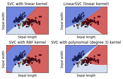
SVC與LinearSVC差別在Hingeloss一個是最小化另一個是平方最小化，可以看出LinearSVC的效果似乎好些。當然非線性的效果一定更好poly是多項式，這邊比較特別要提的是rbf可以看出它已經像在畫太極了＠＠

RBF 徑向核函數

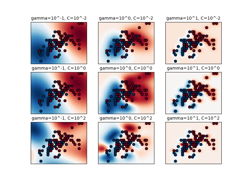
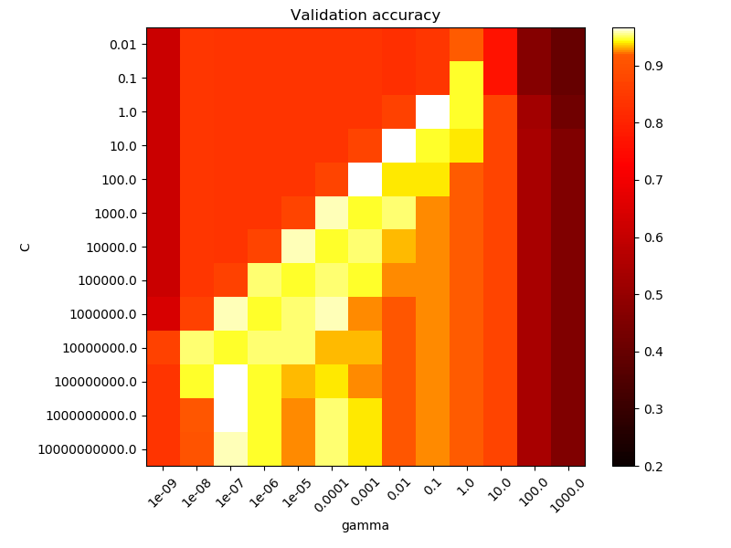
rbf(Radial Based Function)徑向核函數它可以表示無限多維空間，這邊稍微解釋gamma與Ｃ的參數意義。code就不貼上了，直接從底下的圖可以看出gamma值如果愈大資料點影響的範圍愈小，Ｃ值愈大outlier忍受程度愈小，從左下圖可以發現原本藍色區域只要有一點紅色資料點參雜就會使系統判定藍色範圍劇烈減少。那如何找出適合的gamma與Ｃ值？其實就是暴力法地毯式搜索下圖就是利用accuracy做一個gammar與Ｃ的gridserch，通常大於0.92就很不錯了。