
今天從Inside Airbnb下載的資料(listing.csv),針對德國柏林地區的Airbnb房源初步分析。
The data (listing.csv) was collected from Inside Airbnb, the data was last updated on 11/07/2019.
Today's article will briefly analysise the house listing of Airbnb in Berlin.
# 載入所需套件 import the packages we need
import pandas as pd
import numpy as np
import matplotlib.pyplot as plt # 畫互動式圖表的開源套件 graphing library makes interactive graphs
import seaborn as sns
import plotly as py

import warnings # 忽略警告訊息
warnings.filterwarnings("ignore")
Read in the listing file
listing = pd.read_csv('airbnb/listings.csv') # 讀入listing檔案來分析 read in the listing file
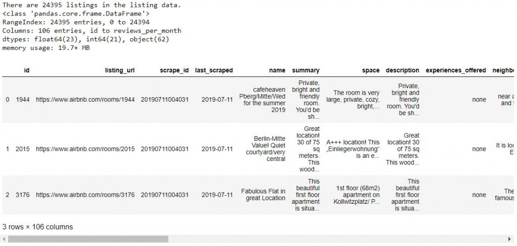
print('There are', listing.id.nunique(), 'listings in the listing data.')
listing.info() # 查看資料細節 the info of data
listing.head(3) # 叫出前三筆資料看看 print out the top three rows of data
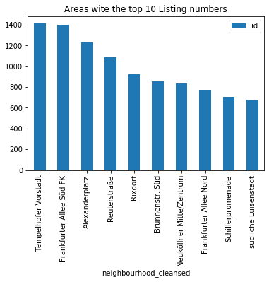
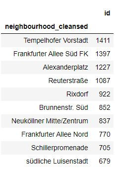
Print out the areas with top ten amounts of listings
# 對數量做排序並只取前10存成grouped_df sort the listing and only save the top 10 listing in to grouped_df
grouped_df = listing.groupby('neighbourhood_cleansed').count()[['id']].sort_values('id', ascending=False).head(10)
grouped_df.plot(kind='bar', title='Areas wite the top 10 Listing numbers')
grouped_df
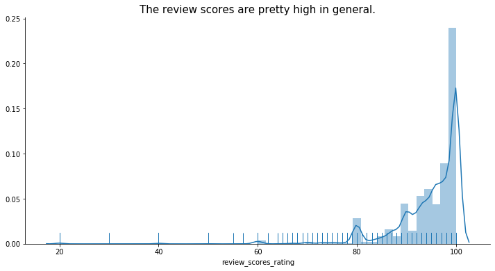
Plot out the review scores
# 去缺失值並畫出顧客評分圖 drop missing values then plot out the review scores
plt.figure(figsize=(12 , 6))
plt.title('The review scores are pretty high in general.', fontsize=15)
sns.distplot(listing.review_scores_rating.dropna(), rug=True)
sns.despine()
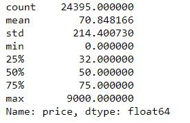
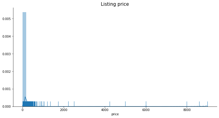
Check out the price range of listings
listing['price'] = listing['price'].astype(str).str.replace(',', '').astype(str).str.replace('$', '').astype(float)

print(listing.price.describe()) # 印出一些價格分布數值 get an intuition of what the data look like
plt.figure(figsize = (12, 6))
plt.title('Listing price', fontsize=15)
sns.distplot(listing.price.dropna(), rug=True)
sns.despine()
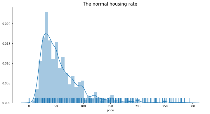
Plot without outliers
# 去除離群值 plot without outliers
plt.figure(figsize=(12 , 6))
plt.title('The normal housing rate', fontsize=15)
sns.distplot(listing[listing.price<300].price.dropna(), rug=True)
sns.despine()
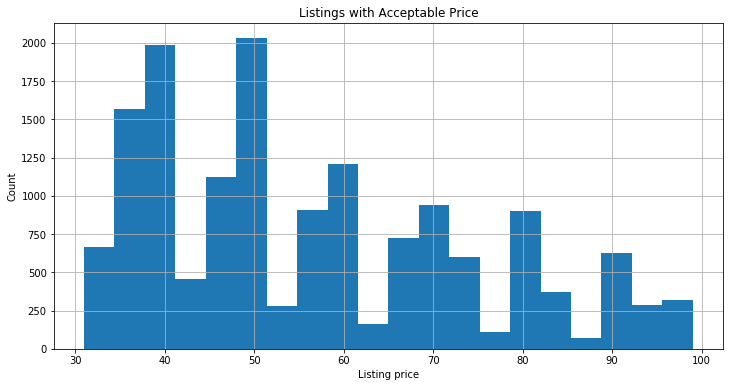
Plot out the data with reasonable price
# 畫出可接受價位區間的資料 plot out the data with reasonable price
plt.figure(figsize=(12,6))
listing.loc[(listing.price<100)&(listing.price>30)].price.hist(bins=20)
plt.ylabel('Count')
plt.xlabel('Listing price')
plt.title('Listings with Acceptable Price')
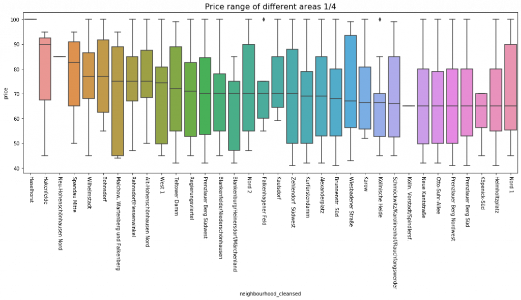
Plot out price range of different areas
drop_outlier_price_condition = listing.loc[(listing.price<=100)&(listing.price>40)]
sort_price = drop_outlier_price_condition\
.groupby('neighbourhood_cleansed')['price']\
.median()\
.sort_values(ascending=False)\
.index
# 柏林共133的區域,由於區域眾多,先分四圖表畫出來看看
# due to the large numbers of areas in Berlin(133), plotted into 4 plots.
plt.figure(figsize=(18,6))
plt.title('Price range of different areas 1/4', fontsize=16)
sns.boxplot(y='price', x='neighbourhood_cleansed', data=drop_outlier_price_condition, order=sort_price[:34])
plt.xticks(rotation=-90)
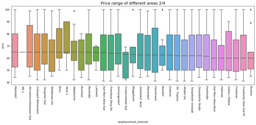
plt.figure(figsize=(18,6))
plt.title('Price range of different areas 2/4', fontsize=16)
sns.boxplot(y='price', x='neighbourhood_cleansed', data=drop_outlier_price_condition, order=sort_price[34:67])
plt.xticks(rotation=-90)
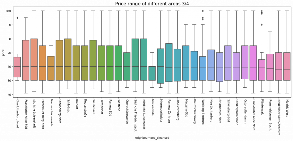
plt.figure(figsize=(18,6))
plt.title('Price range of different areas 3/4', fontsize=16)
sns.boxplot(y='price', x='neighbourhood_cleansed', data=drop_outlier_price_condition, order=sort_price[67:100])
plt.xticks(rotation=-90)
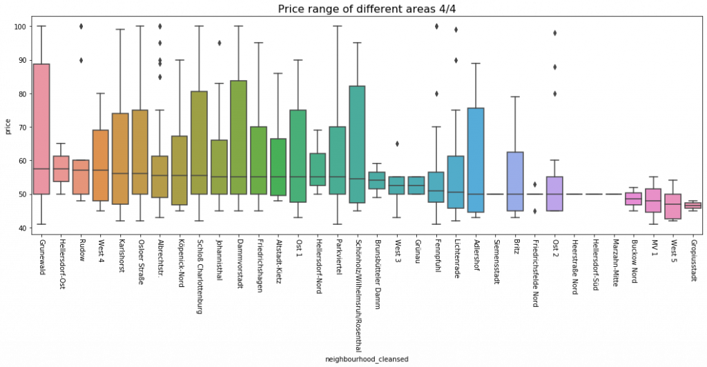
plt.figure(figsize=(18,6))
plt.title('Price range of different areas 4/4', fontsize=16)
sns.boxplot(y='price', x='neighbourhood_cleansed', data=drop_outlier_price_condition, order=sort_price[100:])
plt.xticks(rotation=-90)
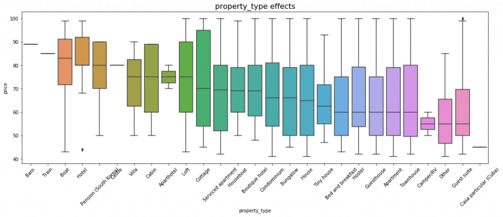
The relation between different property types and price
def boxplot_to_price(category_name):
    sort_price = drop_outlier_price_condition\
                .groupby(category_name)['price']\
                .median()\
                .sort_values(ascending=False)\
                .index
    plt.figure(figsize=(18,6))
    plt.title(category_name +' effects', fontsize=16)
    sns.boxplot(y='price', x=category_name, data=drop_outlier_price_condition, order=sort_price)
    plt.xticks(rotation=45)
boxplot_to_price('property_type')
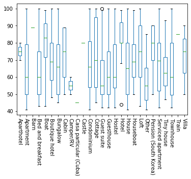
drop_outlier_price_condition.pivot(columns='property_type', values='price').plot(kind='box')
plt.xticks(rotation=-90)
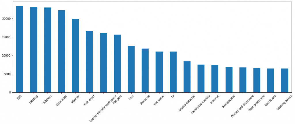
The top 20 amenities listings contain
listing['amenities'] = listing.amenities.str.replace('[{}]', '').str.replace('"', '')
listing.amenities.head()
all_item_ls = np.concatenate(listing.amenities.map(lambda am:am.split(',')))
Top20_item = pd.Series(all_item_ls).value_counts().head(20)
plt.figure(figsize=(18 , 6))
Top20_item.plot(kind='bar')
plt.xticks(rotation=45)
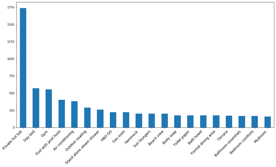
The bottom 20 amenities listings contain
amenities = np.unique(np.concatenate(listing['amenities'].map(lambda amns: amns.split(","))))
amenity_prices = [(amn, listing[listing['amenities'].map(lambda amns: amn in amns)]['price'].mean()) for amn in amenities if amn != ""]
amenity_srs = pd.Series(data=[a[1] for a in amenity_prices], index=[a[0] for a in amenity_prices])
plt.figure(figsize=(16,8))
amenity_srs.sort_values(ascending=False)[:20].plot(kind='bar')
ax = plt.gca()
ax.set_xticklabels(ax.get_xticklabels(), rotation=45, ha='right', fontsize=12)
plt.show()
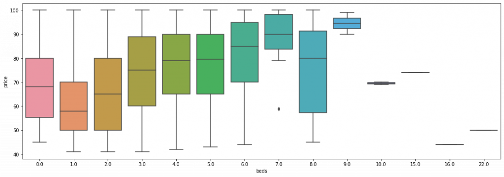
The relation between nembers of beds and price.
plt.figure(figsize=(18,6))
sns.boxplot(y='price', x='beds', data=drop_outlier_price_condition)
plt.show()
本日文章針對柏林房源先有個初步認識,接下來幾篇文章再進一步分析。
Today we briefly walked through the listing data of Airbnb listings in Berlin, in the following articles, we will step a little deeper into analysing the listings.
本篇程式碼請參考Github。The code is available on Github.
文中若有錯誤還望不吝指正,感激不盡。
Please let me know if there’s any mistake in this article. Thanks for reading.
Reference 參考資料:
[1] Inside Airbnb
[2] 利用Airbnb來更了解居住城市,以臺北為例 Python實作(上)

 iThome鐵人賽