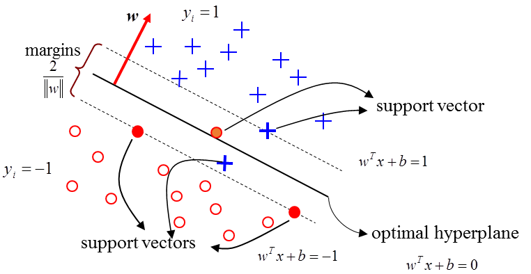
SVM是一種監督式的學習方法，它的基礎的概念非常簡單，就是找到一個決策邊界(decision boundary)讓分類之間的邊界(margins)達到最大，將資料完美分開。
下面圖中有三條直線，都可以將這兩組資料做完美的分割，但綠色直線，特別完美地將這組資料做分割，因為藍色線及紅色線都離這些資料點太近。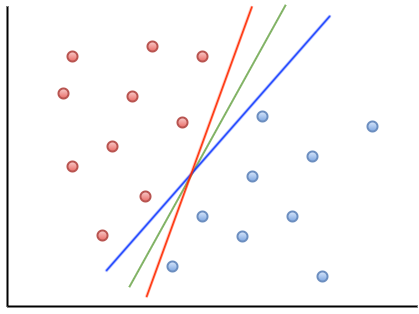

SVM數學推導
兩向量做內積，其意義為把其中一向量投影至另一向量上。以下面這張圖所示，我們把向量v投影至向量u（如果有修過離散數學或工程數學這應該很好理解），p就是我們投影到另一個向量上的長度。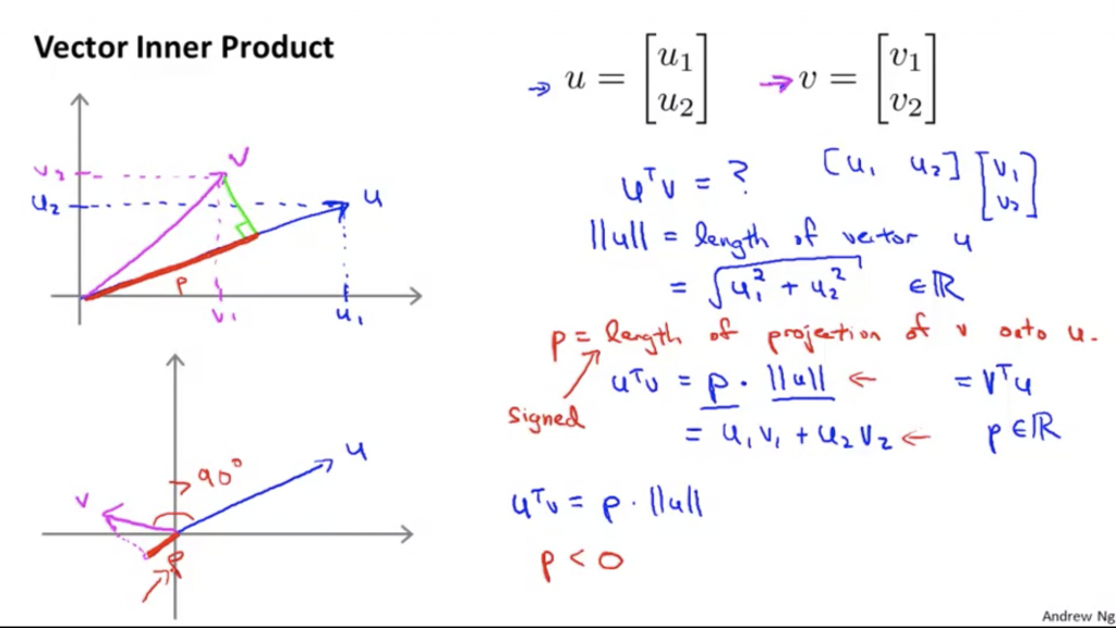

我們要優化的目標函數為1/2θ²（因為採用吳恩達老師教學影片，θ就是大部分書籍裡的w），這邊以向量內積來解釋θ^Tx，也就是把x投影至向量θ上。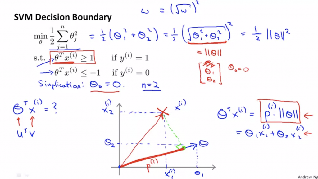

下面這張圖可以看到，左邊的x投影到向量θ上，產生的p非常小，所以會造成θ的範數（長度的概念）非常大，這與我們要優化的目標函數產生矛盾；反之，右邊的x投影到向量θ上，產生的p非常大，所以會造成θ的範數（長度的概念）非常小，符合我們的目的，其中左右兩邊最靠近決策邊界的p值就是所謂的margin。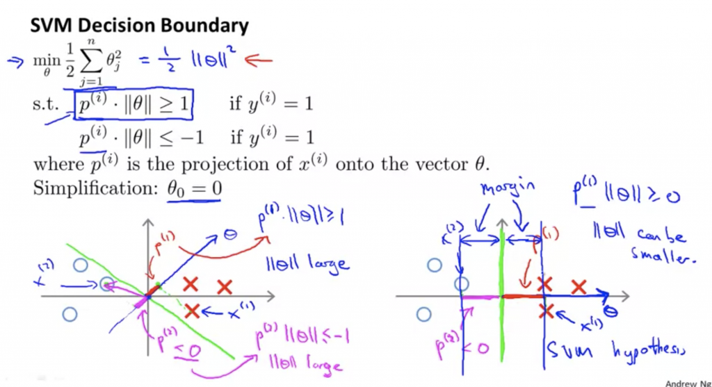

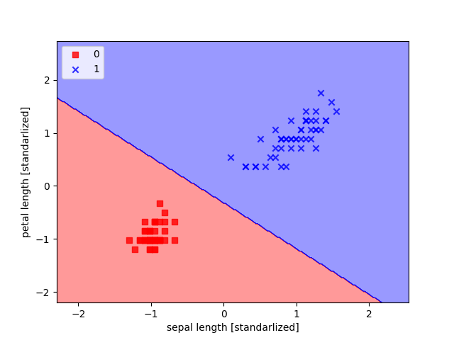
鳶尾花程式碼實作

import matplotlib.pyplot as plt
from sklearn import datasets
import numpy as np
from sklearn.preprocessing import StandardScaler
from sklearn.model_selection import train_test_split
from sklearn.svm import SVC
from sklearn.metrics import accuracy_score
from matplotlib.colors import ListedColormap


def plot_decision_regions(X, y, classifier, test_idx=None, resolution=0.02):
    # setup markers generator and color map
    markers = ('s', 'x', 'o', '^', 'v')
    colors = ('red', 'blue', 'lightgreen', 'gray', 'cyan')
    cmap = ListedColormap(colors[:len(np.unique(y))])

    # plot the decision surface
    x1_min, x1_max = X[:, 0].min() - 1, X[:, 0].max() + 1
    x2_min, x2_max = X[:, 1].min() - 1, X[:, 1].max() + 1
    xx1, xx2 = np.meshgrid(
        np.arange(x1_min, x1_max, resolution),
        np.arange(x2_min, x2_max, resolution))

    z = classifier.predict(np.array([xx1.ravel(), xx2.ravel()]).T)
    z = z.reshape(xx1.shape)
    plt.contourf(xx1, xx2, z, alpha=0.4, cmap=cmap)
    plt.xlim(xx1.min(), xx1.max())
    plt.ylim(xx2.min(), xx2.max())

    # plot all samples
    X_test, y_test = X[test_idx, :], y[test_idx]
    for idx, cl in enumerate(np.unique(y)):
        plt.scatter(
            x=X[y == cl, 0],
            y=X[y == cl, 1],
            alpha=0.8,
            c=cmap(idx),
            marker=markers[idx],
            label=cl)

    # hightlight test samples
    if test_idx:
        X_test, y_test = X[test_idx, :], y[test_idx]
        plt.scatter(
            X_test[:, 0],
            X_test[:, 1],
            c='',
            alpha=1.0,
            linewidth=1,
            marker='o',
            s=55)


def main():
    iris = datasets.load_iris()
    X = iris.data[:, [2, 3]]
    y = iris.target
    X = np.array([m for m, n in zip(X, y) if n != 2])
    boolarr = y != 2
    y = y[boolarr]

    X_train, X_test, y_train, y_test = train_test_split(
        X, y, test_size=0.3, random_state=0)

    sc = StandardScaler()
    sc.fit(X_train)
    X_train_std = sc.transform(X_train)
    X_test_std = sc.transform(X_test)

    svm = SVC(kernel='linear', C=1.0, random_state=0)
    svm.fit(X_train_std, y_train)
    y_pred = svm.predict(X_test_std)

    print("Misclassified smaples: %d" % (y_test != y_pred).sum())
    print("Accuracy: %0.2f" % accuracy_score(y_test, y_pred))

    X_combined_std = np.vstack((X_train_std, X_test_std))
    y_combined_std = np.hstack((y_train, y_test))
    plot_decision_regions(
        X=X_combined_std,
        y=y_combined_std,
        classifier=svm,
        test_idx=range(50, 100))
    plt.xlabel('sepal length [standarlized]')
    plt.ylabel('petal length [standarlized]')
    plt.legend(loc='upper left')
    plt.show()


if __name__ == "__main__":
    main()