
在模型更新時,我們可以利用 損失函數 (cost function) 來得到誤差,再來我們會根據這個函數的微分去做權重更新,而權重值更新的策略如何,就是看你使用了怎麼樣的優化器 (optimizer),那這個優化器在 tensorflow 裡又該如何使用呢?且每個不同的優化器個代表什麼意義呢?今天來為大家介紹!
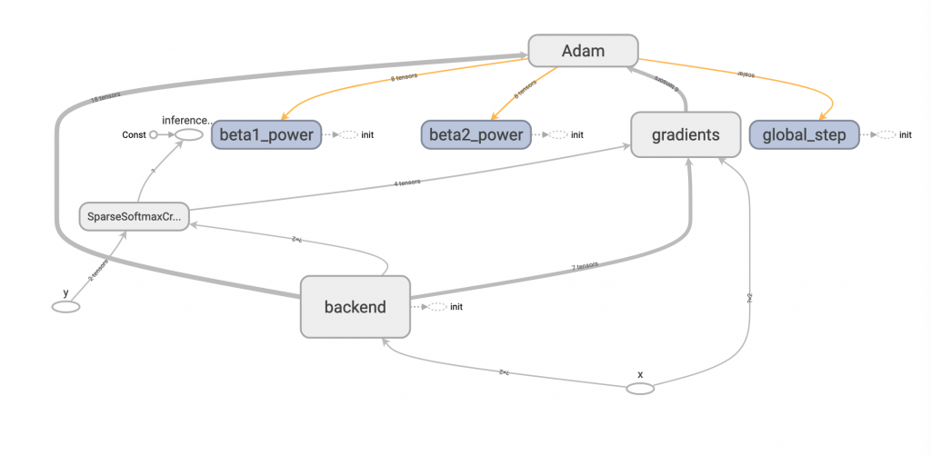
首先,我們假定要處理一個分類問題,所以會用 tf.nn.sparse_softmax_cross_entropy_with_logits ,作為損失函數,最前面程式碼我這樣規劃。
global_step = global_step = tf.train.get_or_create_global_step()

x = tf.placeholder(shape=[None, 2], dtype=tf.float32, name='x')
y = tf.placeholder(shape=[None], dtype=tf.int32, name='y')

with tf.variable_scope('backend'):
   net = tf.layers.dense(x, 64, activation=tf.nn.relu6,
                               kernel_initializer=WEIGHT_INIT,
                               bias_initializer=BIAS_INIT,
                               kernel_regularizer=REGULARIZER,
                               bias_regularizer=REGULARIZER,
                               name='dense_1')
   net = tf.layers.dense(net, 64, activation=tf.nn.relu6,
                               kernel_initializer=WEIGHT_INIT,
                               bias_initializer=BIAS_INIT,
                               kernel_regularizer=REGULARIZER,
                               bias_regularizer=REGULARIZER,
                               name='dense_2')
   logits = tf.layers.dense(net, 2, kernel_initializer=WEIGHT_INIT,
                               bias_initializer=BIAS_INIT,
                               kernel_regularizer=REGULARIZER,
                               bias_regularizer=REGULARIZER,
                               name='final_dense')

loss = tf.reduce_mean(
   tf.nn.sparse_softmax_cross_entropy_with_logits(
       logits=logits, labels=y), name='inference_loss')
然後特別寫了一個方法來決定要使用哪種優化器。
def get_optimizer(opt_type):
   if opt_type == 'gd':
       return tf.train.GradientDescentOptimizer(learning_rate=0.1)
   if opt_type == 'momentum':
       return tf.train.MomentumOptimizer(learning_rate=0.1, momentum=0.9)
   if opt_type == 'ada_grad':
       return tf.train.AdagradOptimizer(learning_rate=0.1, initial_accumulator_value=0.1)
   if opt_type == 'rmsp':
       return tf.train.RMSPropOptimizer(learning_rate=0.1, decay=0.9, momentum=0)
   if opt_type == 'adam':
       return tf.train.AdamOptimizer(learning_rate=0.1, beta1=0.9, beta2=0.99)
在選定完優化器後,我們可以幫此優化器綁定 global_step,如此只要 train_op 執行過一次,不只會更新權重,同時也會自動幫 global_step 加一。
opt = get_optimizer(opt_type)

grads = opt.compute_gradients(loss)
train_op = opt.apply_gradients(grads, global_step=global_step)
再來,就是這次的資料集,為了方便 demo ,我寫了一個座標位置 xor 的方法來當測試,內容很簡單,他會產生 batch 為 16 的二維坐標,其座標值在 -1~1 之間 (遇到 0 就算了),然後在第一和第三象限的座標結果值為 0,二和四象限的座標結果值為 1,兩行搞定。
def get_xor_data():
   x = (np.random.rand(16, 2) - 0.5) * 2
   y = [0 if 0 < x1 * x2 else 1 for x1, x2 in x]

   return x, y
我們訓練 100 次,並記錄所花費的時間,大家就可以自己比較各個不同優化器的收斂速度。
with tf.Session() as sess:
   sess.run(tf.global_variables_initializer())
   sess.run(tf.local_variables_initializer())

   start = timeit.default_timer()
   for _ in range(0, 100):
       x_v, y_v = get_xor_data()
       _, count = sess.run([train_op, global_step], feed_dict={x: x_v, y: y_v})

       print(f'iter: {count}')

   print(f'done. cost {timeit.default_timer() - start} sec.')
結果圖: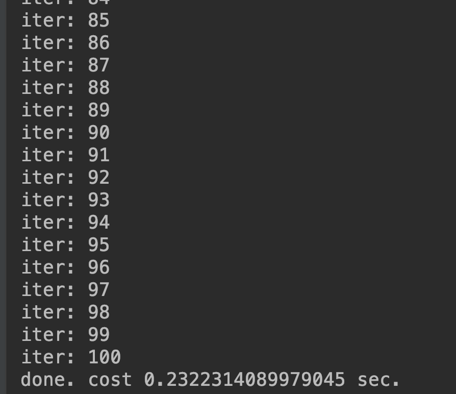
tensorflow 幫我們做了那麼多種優化器,用起來是很方便,但是你真的懂每個優化器使用時機嗎?沒錯,這次我也想挑戰以自己的話來解釋這幾種優化器的差異!
一、GradientDescentOptimizer
tf.train.GradientDescentOptimizer(learning_rate=0.1)
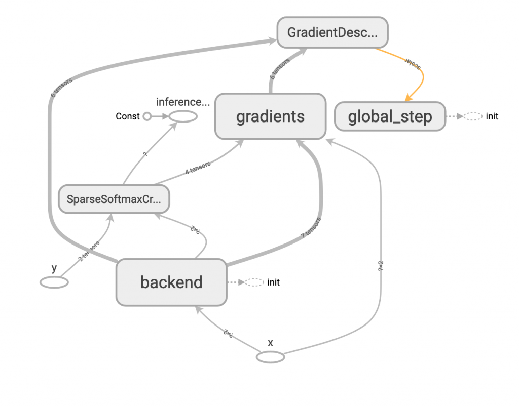
這個應該大家都知道,即最基本的 gradient descent,所需參數僅需要學習速度 learning rate。
對 cost function (以 J 表示) 的微分式子如下,t 表示某 step,theta 表示權重值。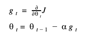
所以權重的更新就可以表示成(式子的 alpha 就是 learning rate):
二、MomentumOptimizer
tf.train.MomentumOptimizer(learning_rate=0.1, momentum=0.9)
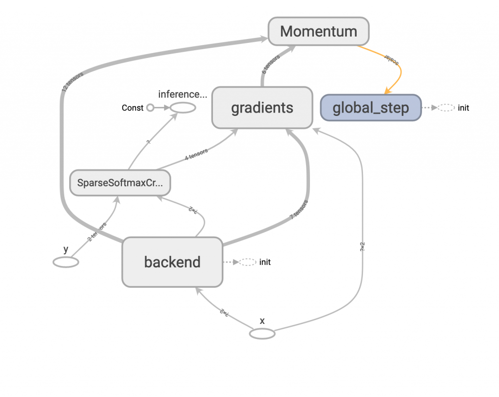
這個方法多了 momentum 這個參數,這個值通常設為 0.9 或 0.99,代表這次的更新量有多少部分是參考前一次的值,從公式上來理解可以比較清楚。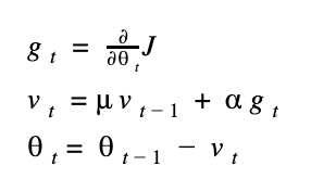
mu (很像 u 的符號) 表示 momentum 的參數值,v 表示目前更新值的大小,因此當模型開始訓練時,每次的更新量會被之前的更新量牽制,比較不容易忽大忽小,以增加穩定性。
三、AdagradOptimizer
tf.train.AdagradOptimizer(learning_rate=0.1, initial_accumulator_value=0.1)
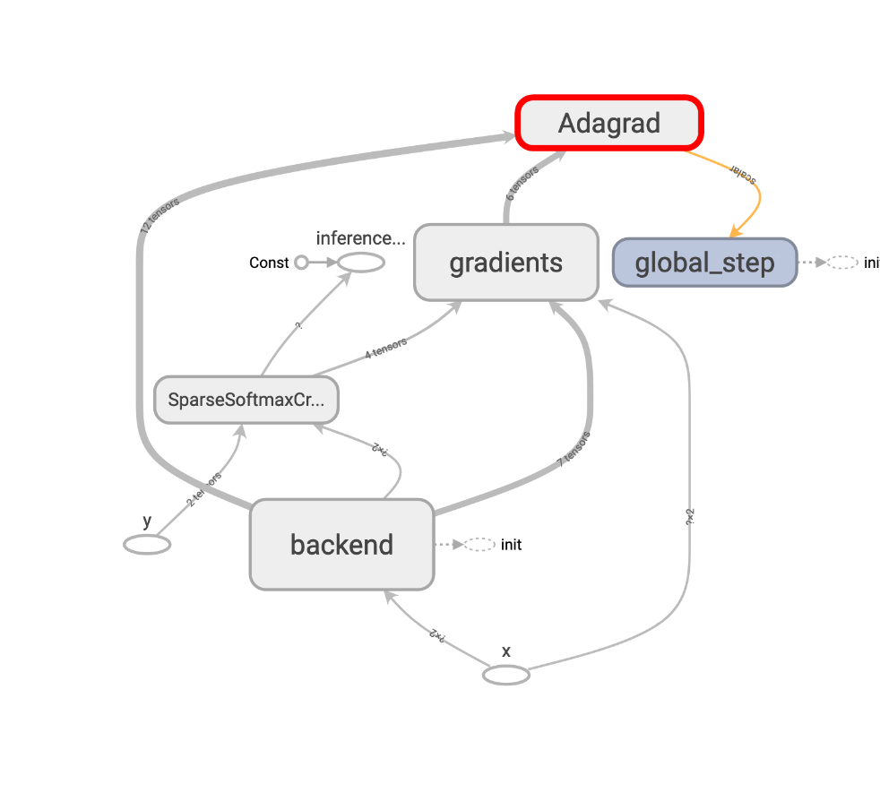
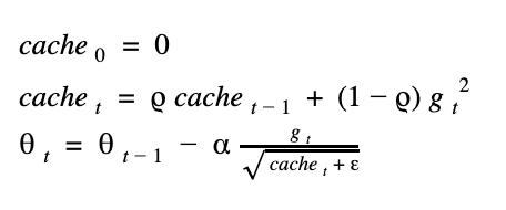
這是以另一種想法來更新權重,我們用了一個會慢慢累加的快取 (cache),來實作,我們將這個 cache 初始值設為 0.1 ,我們來看公式:
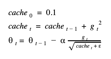
由於 gradient 的值會平方,所以保證 cache 一定是正數,可以放心開根號,但有些框架會預設把 cache 起始值設為0,那第一次迭代時,就有可能發生對0開根號的窘狀,所以會在公式中補個很小的 epsilon 來避免。
仔細想想,這樣的公式前其後和其會有什麼差異?訓練前期時,因為 cache 很小 又放在分母, gradient 除上這個值後會增大,因此更新量也大,訓練到後期時,cache 增大,gradient 除上大數字後,會讓更新量變小,因此牽制了後期的訓練量,使它越來越穩定。
四、RMSPropOptimizer
tf.train.RMSPropOptimizer(learning_rate=0.1, decay=0.9, momentum=0)
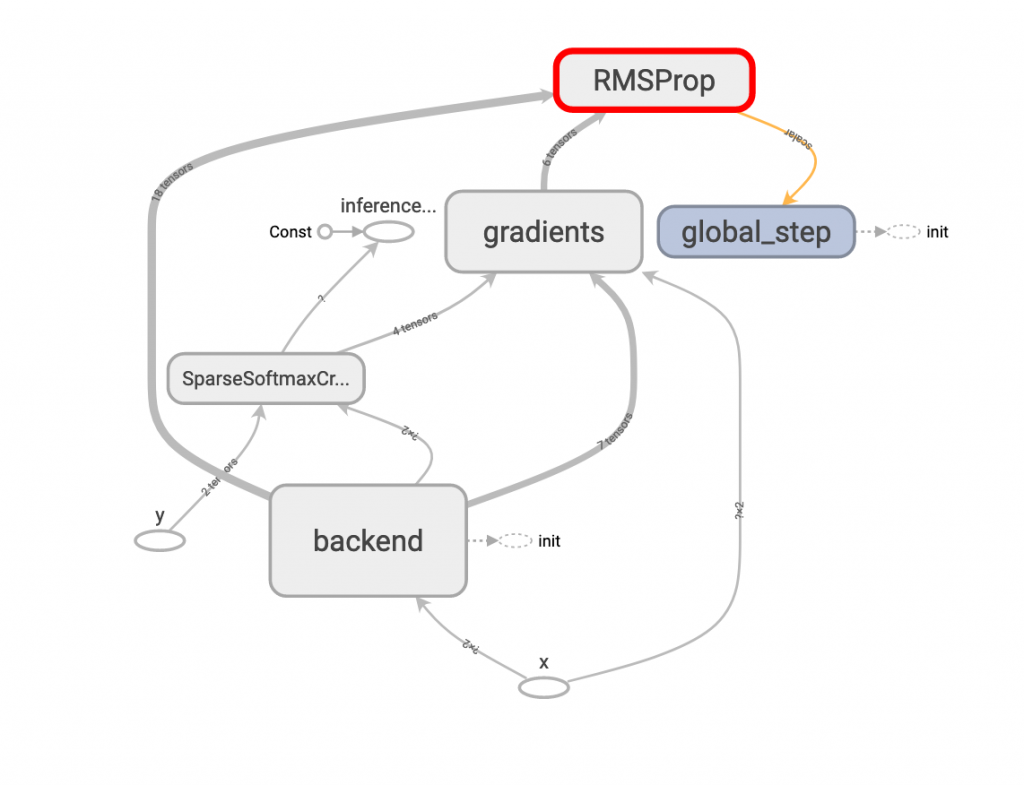
rmsprop 其實很簡單,它只比上面 adagrad 多了decay 的概念,所以有了 decay 這個參數,通常為 0.9 或 0.99,公式如下:
公式和 adagrad 幾乎一樣,只是多了一個 decay 值(這邊表示為 rho 很像 p 的符號),那這個 rho 代表什麼意義呢?沒錯,它跟 momentum 很像,都代表著這次的 cache 值用多少部分的前一次的 cache 值加上這次的 gradient 值,設成 0.99 就是要用 99% 的前一次 cache 來更新。
而 tensorflow 的 API中多了 momentum 參數可以指定,其意義和前面介紹的 momentum 意思相同,但這邊為了專注解釋 rmsprop 所以就不多贅述。
五、AdamOptimizer
tf.train.AdamOptimizer(learning_rate=0.1, beta1=0.9, beta2=0.99)
如果讀者之前有讀過其他 adam 有關的教學,八成都會提到 adam 是 momentum 加 rmsprop 兩者的方法,呃...在這邊我想說的是,這並不那麼精確,如果是這兩種方法的總和,那上面 tensorflow 的 RMSPropOptimizer 就已經有 momentum 可以用了。那話說回來,這和 adam 有什麼不一樣的地方呢?那就是 adam 多了 bias corrections 這個用法,我們慢慢分解公式。
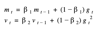
前面提到的 momentum 和 rmsprop 個別都有參數 mu 和 rho 的 decay 概念來控制,在 adam 中,我們個別將其改名 beta1 和 beta2,然後又因為這個公式很剛好又可以被表示成統計學的一二級動差,所以我們換成 mean (公式中的m)和 var (公式中的v)來表示。
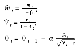
上面戴帽子m 和帽子v 就是經過 bias corrections 的參數,如果你觀察 bias corrections 的公式,可以發現初期 t 很小時,beta1 和 beta2 會把 m 和 v 校正成比較大的參數,以便放大初期的學習效果,等到訓練到後期時,t 慢慢變大,因為 beta1 和 beta2 兩個都是小於1的參數,經過多次方後會超級小,最後根本帽子m 和帽子v 等同於原本的m 和 v (即不校正),所以更新又會趨緩讓模型變得穩定。
看完以上五種方法,大家應該有發現不管哪種方法,都是希望訓練初期可以讓模型走大步一點以加速收斂,直到訓練中後期再慢慢趨緩,避免損失震盪。
呼!為了這篇文,我在 google doc 打了好久的公式,這是我很用心的一篇,自己也花了不少時間把網路上零散的知識一次整理好,如果喜歡還請按個讚,也歡迎提問!

 iThome鐵人賽