使用BigQuery與Datalab進行資料分析(下)

今天的文章將和各位展示一個結合使用BigQuery與Datalab進行資料分析的簡單範例。首先在這裡簡單介紹BigQuery的使用，我們將使用的是課程提供的學習平台Qwiklabs，我們可以藉由此學習平台提供的Google Cloud Platform環境來進行功能的操作。

進入Google Cloud Platform的介面後，在右手邊的選單中，我們找到BigQuery之後(見圖1)，進行點擊，便可進入BigQuery的使用介面(見圖2)，在此使用介面上，最主要可以看到輸入SQL查詢語句(Query editor)與執行的地方(Run)。在這裡，我們試運行一個範例語句，假設我們想知道一個航班資料集中，各個出發機場與抵達機場間的航班數量加總，我們可以使用以下SQL語句:

SELECT
  departure_airport,
  arrival_airport,
  COUNT(1) AS num_flights
FROM
  `bigquery-samples.airline_ontime_data.flights`
GROUP BY
  departure_airport,
  arrival_airport
ORDER BY
  num_flights DESC
LIMIT
  10

經由執行以上語句後，便可得到如圖3當中的結果。且在經過瞭解此資料集後，發現資料集雖然有高達7000多萬的列數目與17個欄位數，卻仍能在短時間內得到結果，可見BigQuery功能的強大之處。

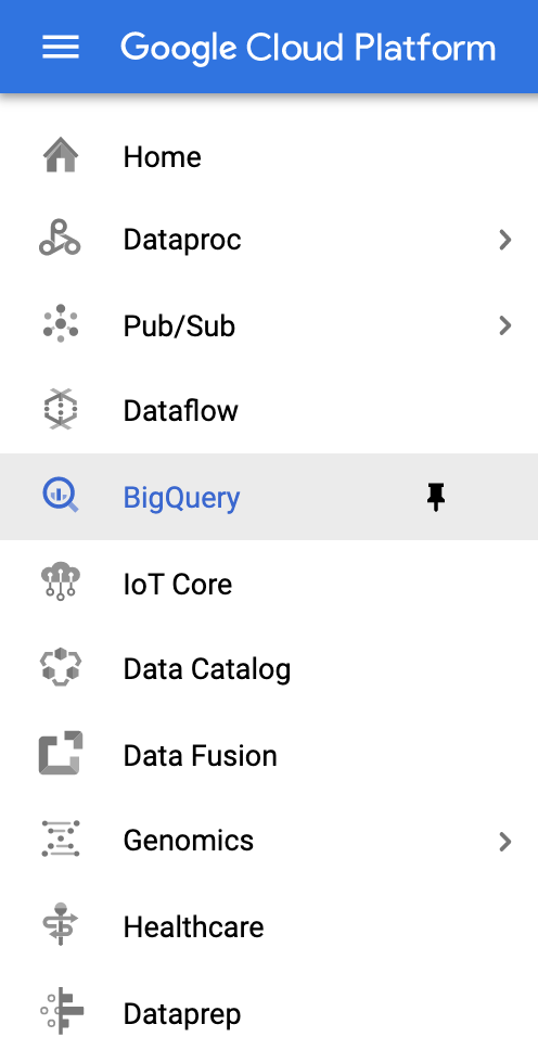
圖1
Source: Coursera - How Google does Machine Learning, Qwiklabs

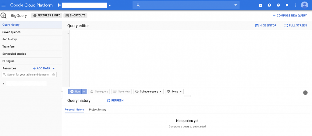
圖2
Source: Coursera - How Google does Machine Learning, Qwiklabs

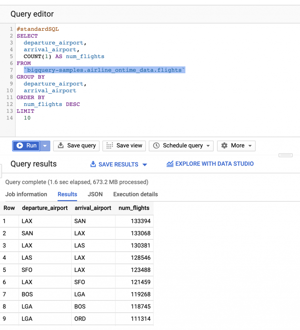
圖3
Source: Coursera - How Google does Machine Learning, Qwiklabs

接著我們再使用Datalab進行資料分析，在經過一些設定後，我們打開了Datalab，並新增一個新的Notebook，映入眼簾的就是大家熟悉的Jupyter Notebook介面。

首先我們使用Python代碼從BigQuery資料庫中擷取我們欲用來進行分析的資料:

query="""
SELECT
  departure_delay,
  COUNT(1) AS num_flights,
  APPROX_QUANTILES(arrival_delay, 10) AS arrival_delay_deciles
FROM
  `bigquery-samples.airline_ontime_data.flights`
GROUP BY
  departure_delay
HAVING
  num_flights > 100
ORDER BY
  departure_delay ASC
"""

import google.datalab.bigquery as bq
df = bq.Query(query).execute().result().to_dataframe()
df.head()

得到了如圖4顯示的輸出結果後，再使用以下Python代碼將分析結果進行更清楚的呈現:

import pandas as pd
percentiles = df['arrival_delay_deciles'].apply(pd.Series)
percentiles = percentiles.rename(columns = lambda x : str(x*10) + "%")
df = pd.concat([df['departure_delay'], percentiles], axis=1)
df.head()

得到了如圖5顯示的輸出結果後，最後再使用以下Python代碼將分析結果藉由Python中Matplotlib套件的視覺化功能，將分析結果繪製出來(見圖6)，以清楚地表達多個變數間的相互關係，讓資料分析工作者得以從中挖掘有價值之洞見。

without_extremes = df.drop(['0%', '100%'], 1)
without_extremes.plot(x='departure_delay', xlim=(-30,50), ylim=(-50,50));

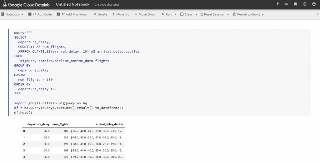
圖4
Source: Coursera - How Google does Machine Learning, Qwiklabs

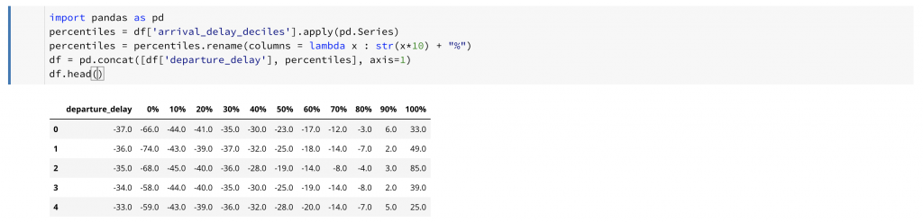
圖5
Source: Coursera - How Google does Machine Learning, Qwiklabs

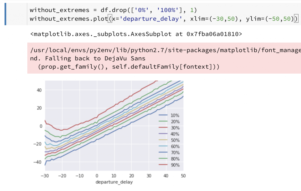
圖6
Source: Coursera - How Google does Machine Learning, Qwiklabs