完整的語音情緒辨識系統流程如圖 1。語音訊號先經過特徵擷取的過程擷取出聲學特徵，再將聲學特徵進行前處理，經過前處理過後的特徵做為分類模型的輸入並進行訓練。分類模型訓練完成之後，再將測試資料輸入至分類模型中得到分類結果。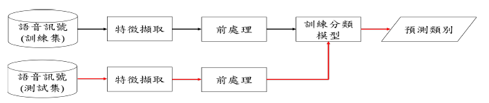

圖 1: 語音辨識系統流程圖。黑色箭頭表示訓練階段，紅色箭頭表示測試階段

實驗中超參數(hyper-parameter)的設定是根據 early-stopping 演算法，我們將原始訓練集的 80% 做為訓練集而剩餘的 20% 做為 early-stopping 演算法需要的驗證集(validation set)。當訓練過程中每一個 epoch 結束時，如果驗證集的損失獲得改善我們就會儲存此次 epoch 的模型參數，當連續 patience 次的訓練與已紀錄的最佳驗證集損失相比都沒有改善的話，訓練就會結束。訓練結束時最後回傳的會是最佳的模型參數(驗證集損失最佳)。
在訓練神經網路時設定的超參數如表 1，其中，optimizer的部份採用 adam 與 sgd，主要的差別在於訓練過程中 adam 的收斂速度較快，因此訓練次數會較少；而 sgd 收斂速度較慢，因此訓練次數會較多。

hyper-parameter	value
mini-batch	100
learning rate	0.002
learning rate decay	0.00001
optimizer	(1) adam (2) sgd
loss function	cross-entropy
patience	3
表 1: 模型超參數
learning rate decay 的公式如下:

首先先對靜態模型進行說明，我們會採用 MLP (Multilayer Perceptron) 與 CNN 兩種架構。
MLP 的架構如下圖 2: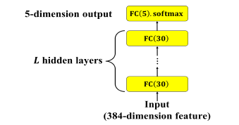

圖 2: MLP 靜態模型。L 表示隱藏層層數
輸入為 Day20 時說明過的 384 維的特徵向量，隱藏層為 30 個神經元並採用兩種 activation function (tanh、ReLU) 的全連接層 (Fully Connected, FC)，共有 L 層，輸出層為 5 個神經元的全連接層，activation function為 softmax。不同層數與不同激活函數的實驗結果比較如表 2。

Activation function 參考：https://himanshuxd.medium.com/activation-functions-sigmoid-relu-leaky-relu-and-softmax-basics-for-neural-networks-and-deep-8d9c70eed91e

hidden layers (L) | UA recall (tanh) | UA recall (ReLU)
------------- | -------------
1 | 46.0% | 45.5%
2 | 46.2% | 45.9%
3 | 45.9% | 45.4%
表2: 不同層數及不同activation function MLP 結果比較

從表中可發現網路架構的深度與 UA recall 並非成正比關係，兩層隱藏層的表現要比三層來的更好。主要原因應為訓練集的資料量並不多，因此如果模型複雜度太高反而會使模型在訓練集上產生過擬合(overfitting)的現象。
程式的部分如下：

import os
os.environ['TF_CPP_MIN_LOG_LEVEL'] = '3'
import tensorflow as tf
import numpy as np
import argparse
import math

from keras.layers import *
from keras.models import *
from keras.optimizers import SGD, Adam
from keras.callbacks import EarlyStopping, ModelCheckpoint
from keras.layers.merge import *
from utils import *
from keras import backend as K
from keras.models import load_model
from keras.utils import plot_model, print_summary

MODEL_ROOT_DIR = './static_model/'

# Learning parameters
BATCH_SIZE = 100
TRAIN_EPOCHS = 10
LEARNING_RATE = 0.002
DECAY = 0.00001
MOMENTUM = 0.9
# Network parameters
CLASSES = 5 # A,E,N,P,R
LLDS = 16
FUNCTIONALS = 12
DELTA = 2
STATIC_FEATURES = LLDS*FUNCTIONALS*DELTA
HIDDEN_UNITS = 30
USE_TEACHER_LABEL = 0



def train_MLP(train_data, train_label, train_size, test_data, test_label, test_size):
	args = get_arguments()
	data_weights = []
	data_weights.append([1.1,0.5,0.2,1.5,1.4])
	data_weights = np.asarray(data_weights)
	class_weight = {0: 1.1, 1: 0.5, 2: 0.2, 3: 1.5, 4: 1.4}

	# 16x12x2
	mlp_input = Input(shape=[args.static_features], dtype='float32', name='mlp_input')
	hidden_1 = Dense(units=30, activation='relu', name='hidden1')(mlp_input)
	hidden_2 = Dense(units=30, activation='relu', name='hidden2')(hidden_1)
	hidden_3 = Dense(units=30, activation='relu', name='hidden3')(hidden_2)
	output = Dense(units=5, activation='softmax', name='output')(hidden_3)
	model = Model(inputs=mlp_input, outputs=output)
	model.summary()

	if args.load_model == '':
		adam = Adam(lr=args.learning_rate, decay=args.decay)
		model.compile(loss=weighted_loss(r=data_weights), optimizer=adam, metrics=['accuracy'])
		earlystopping = EarlyStopping(monitor='loss', min_delta=0, patience=0)
		checkpoint = ModelCheckpoint(filepath='static_model/mlp_checkpoint.hdf5', monitor='val_loss', save_best_only=True)
		callbacks_list = [earlystopping, checkpoint]
		history = model.fit(x=train_data, y=train_label, batch_size=args.batch_size, epochs=args.train_epochs, verbose=2, 
							  callbacks=callbacks_list)  
		# save the model
		model.save_weights(args.model_root_dir + 'model.h5')
	else:
		print ('Load the model: {}'.format(args.load_model))
		model.load_weights(args.model_root_dir + args.load_model)

	predict = model.predict(test_data, verbose=1)
	show_confusion_matrix(predict, test_label, test_size)

在後續的模型中，我們會針對分類結果較好的其中幾個模型列出混淆矩陣(confusion matrix)來詳細觀察各類別的分類情形。
畫出 confusion matrix 的程式如下:

def show_confusion_matrix(predict, true_label, size):
	num_class = true_label.shape[1]
	AC = np.zeros(num_class)# store the classification result of each class
	AC_WA = 0.0
	AC_UA = 0.0
	confusion_matrix = np.zeros((num_class, num_class))# store the confusion matrix

	for i in range(predict.shape[0]):
		predict_class = np.argmax(predict[i])
		true_class = np.argmax(true_label[i])
		confusion_matrix[true_class][predict_class] += 1
	for i in range(num_class):
		AC[i] = confusion_matrix[i][i] / size[i]

	print("-------------Classification results-------------")
	print ('A: {0} , E: {1} , N: {2} , P:{3} , R: {4}'.format(size[0],size[1],size[2],size[3],size[4]))
	AC_UA = np.mean(AC)
	AC_WA = (confusion_matrix[0][0] + confusion_matrix[1][1] + confusion_matrix[2][2] + confusion_matrix[3][3] + confusion_matrix[4][4] ) / predict.shape[0]
	print('      A      E      N      P      R')
	print('A  %4d   %4d   %4d   %4d   %4d    ' % (confusion_matrix[0][0], confusion_matrix[0][1], confusion_matrix[0][2], confusion_matrix[0][3], confusion_matrix[0][4]))
	print('E  %4d   %4d   %4d   %4d   %4d    ' % (confusion_matrix[1][0], confusion_matrix[1][1], confusion_matrix[1][2], confusion_matrix[1][3], confusion_matrix[1][4]))
	print('N  %4d   %4d   %4d   %4d   %4d    ' % (confusion_matrix[2][0], confusion_matrix[2][1], confusion_matrix[2][2], confusion_matrix[2][3], confusion_matrix[2][4]))
	print('P  %4d   %4d   %4d   %4d   %4d    ' % (confusion_matrix[3][0], confusion_matrix[3][1], confusion_matrix[3][2], confusion_matrix[3][3], confusion_matrix[3][4]))
	print('R  %4d   %4d   %4d   %4d   %4d    ' % (confusion_matrix[4][0], confusion_matrix[4][1], confusion_matrix[4][2], confusion_matrix[4][3], confusion_matrix[4][4]))
	print('\nA: %f    E: %f     N: %f     P: %f     R: %f\n' % (AC[0]*100, AC[1]*100, AC[2]*100, AC[3]*100, AC[4]*100))
	print("WA: {}".format(AC_WA*100))
	print("UA: {}".format(AC_UA*100))
	print("------------------------------------------------")

明天將繼續介紹靜態模型-CNN 部分。