今日大綱

• 程式碼

程式碼

範例所使用的程式碼與支持向量機範例一樣，為分辨真偽鈔來自UCI的資料集

先將需要用到的library與資料匯入

import pandas as pd
from sklearn.model_selection import train_test_split
from sklearn.tree import DecisionTreeClassifier
from sklearn.metrics import confusion_matrix, classification_report
url = 'https://archive.ics.uci.edu/ml/machine-learning-databases/00267/data_banknote_authentication.txt'
columns = ['variance of Wavelet Transformed image', 'skewness of Wavelet Transformed image', 'curtosis of Wavelet Transformed image', 'entropy of image', 'target']
data = pd.read_csv(url, names = columns)

接著，將資料分割成訓練集與測試集

x = data.iloc[:,:-1]
y = data.iloc[:, -1]
x_train, x_test, y_train, y_test = train_test_split(x, y, test_size = 0.2, random_state = 1)

分別訓練利用Gini與Entropy當作切割標準的決策樹

clf_gini = DecisionTreeClassifier(criterion = "gini",
            random_state = 100,max_depth=2)
clf_entropy = DecisionTreeClassifier(criterion = "entropy",
            random_state = 100,max_depth=2)

clf_gini.fit(x_train, y_train)
prediction_gini = clf_gini.predict(x_test)
clf_entropy.fit(x_train, y_train)
prediction_entropy = clf_entropy.predict(x_test)

印出兩個決策樹的結果

from sklearn.metrics import confusion_matrix, classification_report
print("Gini: \n", confusion_matrix(y_test, prediction_gini), classification_report(y_test, prediction_gini))
print("Entropy: \n", confusion_matrix(y_test, prediction_entropy), classification_report(y_test, prediction_entropy))

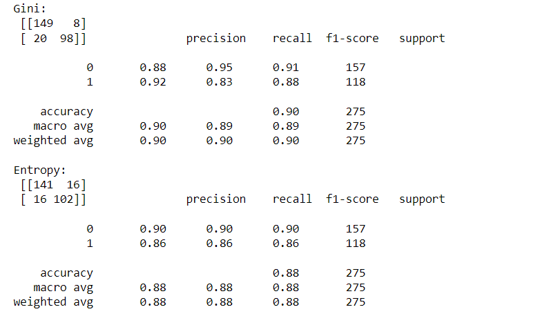
從結果可以發現，利用gini impurity為標準組成的決策樹準確率較高

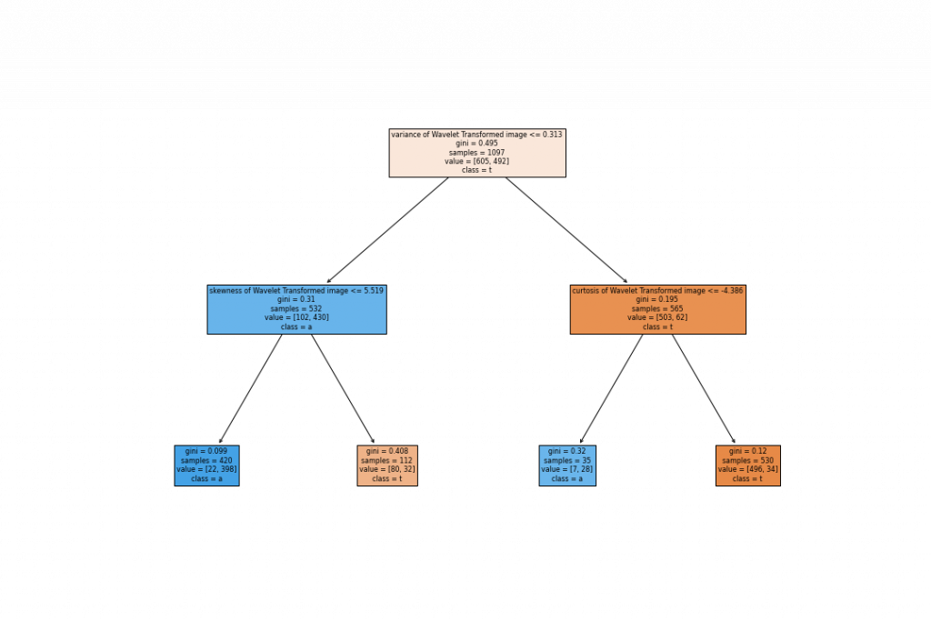
視覺化利用Gini組成的決策樹

import matplotlib.pyplot as plt
from sklearn import tree
fig = plt.figure(figsize=(15,10))
_ = tree.plot_tree(clf_gini, 
                   feature_names=x_train.columns,  
                   class_names='target',
                   filled=True)
fig.savefig("gini.png")

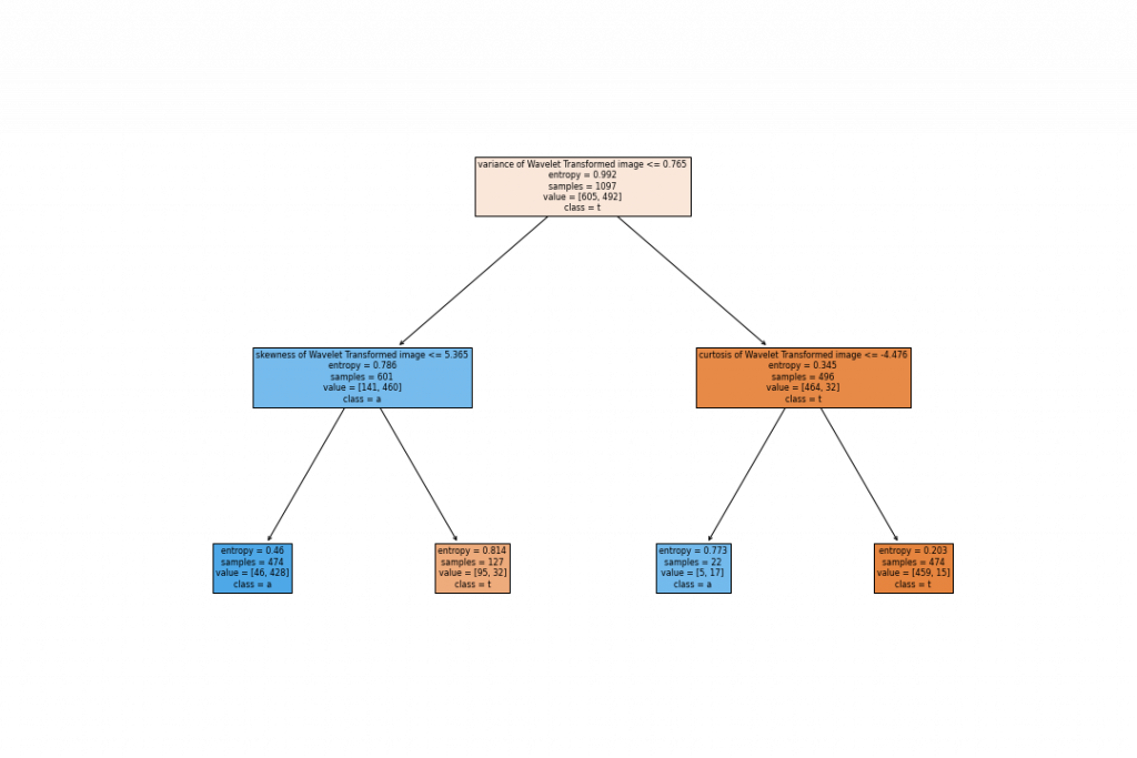
視覺化利用entropy組成的決策樹

fig = plt.figure(figsize=(15,10))
_ = tree.plot_tree(clf_entropy, 
                   feature_names=x_train.columns,  
                   class_names='target',
                   filled=True)
fig.savefig("entropy.png")

最後畫出兩個模型的ROC，並且算出AUC

from sklearn.metrics import roc_curve, roc_auc_score, auc

plt.title('Receiver Operating Characteristic')
# 在各種『決策門檻』（decision threshold）下，計算 『真陽率』（True Positive Rate；TPR）與『假陽率』（False Positive Rate；FPR）
fpr, tpr, threshold = roc_curve(y_test, prediction_gini)
auc = round(roc_auc_score(y_test, prediction_gini), 2)
plt.plot(fpr, tpr, color = 'orange', label = 'Gini_AUC = %0.2f' % auc)
fpr, tpr, threshold = roc_curve(y_test, prediction_entropy)
auc = round(roc_auc_score(y_test, prediction_entropy), 2)
plt.plot(fpr, tpr, color = 'blue', label = 'Entropy_AUC = %0.2f' % auc)

## Plot the result
plt.legend(loc = 'lower right')
plt.plot([0, 1], [0, 1],'r--')
plt.xlim([0, 1])
plt.ylim([0, 1])
plt.ylabel('True Positive Rate')
plt.xlabel('False Positive Rate')
plt.show()

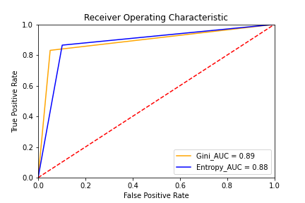
從圖可看出，不管是Accuracy或是AUC，使用Gini impurity的效果比較好。

程式碼已上傳我的Github

參考資料

• Python | Decision tree implementation
• Visualize a Decision Tree in 4 Ways with Scikit-Learn and Python
• How to Plot Multiple ROC Curves in Python (With Example)

感謝您的瀏覽，我們明天見!