今日大綱

• LSTM介紹
• 程式碼

LSTM介紹

RNN存在梯度消失(Vanishing gradient)與梯度爆炸(Exploding gradient)的問題，因此Hochreiter與Schmidhuber在1997年提出長短期記憶網路。

下圖為RNN與LSTM的架構，LSTM多了一個state以及三個閥門。cell state儲存上個神經元的值，而輸入閥(Input gate)決定這個神經元的輸入是否要傳遞下去，遺忘閥(Forget gate)決定之前在cell state裡的值是否要繼續傳遞，輸出閥(Output gate)決定當前輸出是否要輸出。每個閥門的activation function 為sigmoid，以0.5為門檻值判別為0或1。需要特別注意的是，如果遺忘閥的值為0代表遺忘，1代表每個神經元的輸入有三個，分別為當前的特徵值x、上一層的輸出以及上一層cell state裡的值。

各個閥門的公式如下: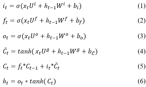

各個閥門特徵值的權重與上一個輸出呈上的權重以及截距項都是透過反項傳播(back probagation)計算的。第一至第三條公式為各個閥門的計算公式，將輸入乘上權重後經過sigmoid函數轉換變成0或1，決定是否將當前的數值傳遞下去。第四條計算與輸入閥相乘的值，先將輸入將過hyperbolic tangent函數轉換，使數值介於1到-1之間。第五條計算cell state更新後的值，而最後一條則為計算輸出值，先將cell state裡的值轉換至1到-1之間，接著與輸出閥的值相乘。

程式碼

今天使用的資料是之前我爬蟲抓取ETtoday的新聞，新聞類別有寵物、健康以及旅遊。新聞我已經完成部分的前處理，接著建立字典，字典裡的單字為5000個，將取頻率出現最高的前5000個單字作轉換。

from tensorflow.keras.preprocessing.text import Tokenizer
import pandas as pd
max_words = 5000
max_len = 500
tokenizer = Tokenizer(num_words=max_words)  ## 使用的最大詞語數為5000
news = pd.read_excel('ETtoday news_202205.xlsx', engine = 'openpyxl')
tokenizer.fit_on_texts(news['tokenization'])

將最常出現的10個單字以及前面10個單字印出

## 使用word_index屬性可以看到每個詞對應的編碼
## 使用word_counts屬性可以看到每個詞對應的頻數
for index,item in enumerate(tokenizer.word_index.items()):
    if index < 10:
        print(item)
    else:
        break
print("===================")  
for index,item in enumerate(tokenizer.word_counts.items()):
    if index < 10:
        print(item)
    else:
        break

將原本新聞類別one-hot encoding轉為數字，並且切割訓練集以及測試集。

from sklearn.preprocessing import OneHotEncoder, LabelEncoder
from sklearn.model_selection import train_test_split
labelencoder = LabelEncoder()
le_y = labelencoder.fit_transform(news['category']).reshape(-1,1)
ohe = OneHotEncoder()
y = ohe.fit_transform(le_y).toarray()
x = news['tokenization']
#Split the data to have 20% validation split
train_x, test_x, train_y, test_y = train_test_split(x, y, test_size=0.2)

將文字轉換為數字，每則新聞最長的長度為500。處理完成後，將資料輸入至LSTM模型訓練。

from sklearn import metrics
from tensorflow.keras.models import Model
from tensorflow.keras.layers import LSTM, Activation, Dense, Dropout, Input, Embedding
from tensorflow.keras.optimizers import RMSprop
from tensorflow.keras.preprocessing.text import Tokenizer
from tensorflow.keras.preprocessing import sequence

train_seq = tokenizer.texts_to_sequences(train_x)
test_seq = tokenizer.texts_to_sequences(test_x)
## 將每個序列調整相同的長度
train_seq_mat = sequence.pad_sequences(train_seq,maxlen=max_len)
test_seq_mat = sequence.pad_sequences(test_seq,maxlen=max_len)
# print(train_seq_mat.shape, test_seq_mat.shape)
inputs = Input(name='inputs',shape=[max_len])
## Embedding(詞匯表大小,vector長度,每個新聞的詞長)
layer = Embedding(max_words+1,128,input_length=max_len)(inputs)
layer = LSTM(128)(layer)
layer = Dense(128,activation="relu",name="FC1")(layer)
layer = Dropout(0.3)(layer)
layer = Dense(3,activation="softmax",name="FC2")(layer)
model = Model(inputs=inputs,outputs=layer)
model.summary()
## multi-classification problem use categorical_crossentropy
model.compile(loss="categorical_crossentropy",optimizer=RMSprop(),metrics=["accuracy"])

model_fit = model.fit(train_seq_mat,train_y,batch_size=128,epochs=10,
                     validation_split=0.2)

檢視訓練的績效

import numpy as np
test_pre = model.predict(test_seq_mat)
## evaluate the performance of prediction
confusion_matrix = metrics.confusion_matrix(np.argmax(test_pre,axis=1),np.argmax(test_y,axis=1))
print("Confusion matrix: \n",confusion_matrix)

scores = model.evaluate(test_seq_mat, test_y, verbose=0)
print("Out-of-sample loss: ", scores[0],"Out-of-sample accuracy:", scores[1])

print(metrics.classification_report(np.argmax(test_pre,axis=1),np.argmax(test_y,axis=1)))

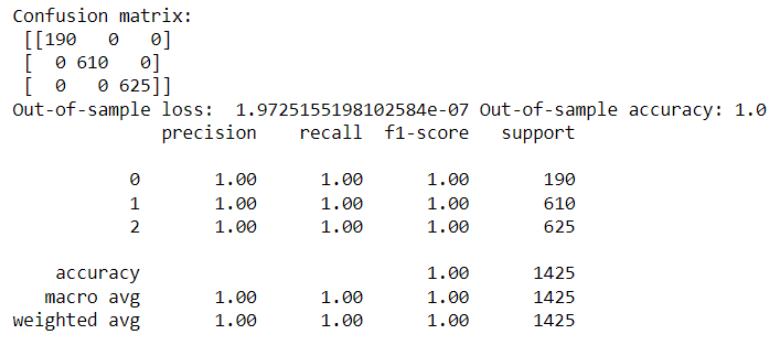
從結果可看出，準確率高達100%，最後檢視測試集與訓練集的準確率、損失值的變化，觀察是否有overfitting。

視覺化準確率與損失值的變化

# 繪製歷程圖
import matplotlib.pyplot as plt
def show_train_history(train_history):
    plt.figure(figsize=(6,5))
    plt.plot(train_history.history['accuracy'])
    plt.plot(train_history.history['val_accuracy'])
    plt.xticks([i for i in range(len(train_history.history['accuracy']))])
    plt.title('Train History')
    plt.ylabel('accuracy')
    plt.xlabel('epoch')
    plt.legend(['Train', 'Val'], loc='upper left')
    plt.savefig('Accuracy.png')
    plt.show()

    plt.figure(figsize=(6,5))
    plt.plot(train_history.history['loss'])
    plt.plot(train_history.history['val_loss'])
    plt.xticks([i for i in range(len(train_history.history['loss']))])
    plt.title('Train History')
    plt.ylabel('loss')
    plt.xlabel('epoch')
    plt.legend(['Train', 'Val'], loc='upper left')
    plt.savefig('Loss.png')
    plt.show()
show_train_history(model_fit)

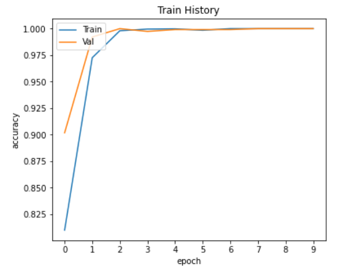
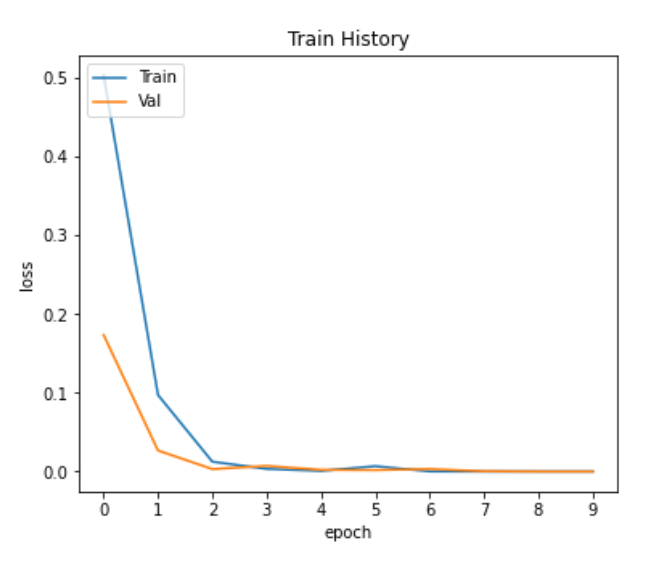
從上面兩張圖可看出，模型並沒有overfitting的情況。

感謝您的瀏覽，程式碼已上傳Github