今日大綱

• GRU介紹
• 程式碼

GRU 介紹

今天將介紹的模型也是RNN的變形，LSTM的簡易版，將遺忘閥(forget gate)與輸入閥(input gate)結合成更新閥(update gate)，並且把cell state與隱藏狀態結合，其算法與原本LSTM已經不同。雖然GRU的作者聲稱，GRU的時間複雜度比LSTM低，但是很多人發現其實相差不遠，而且LSTM比起GRU更常被使用。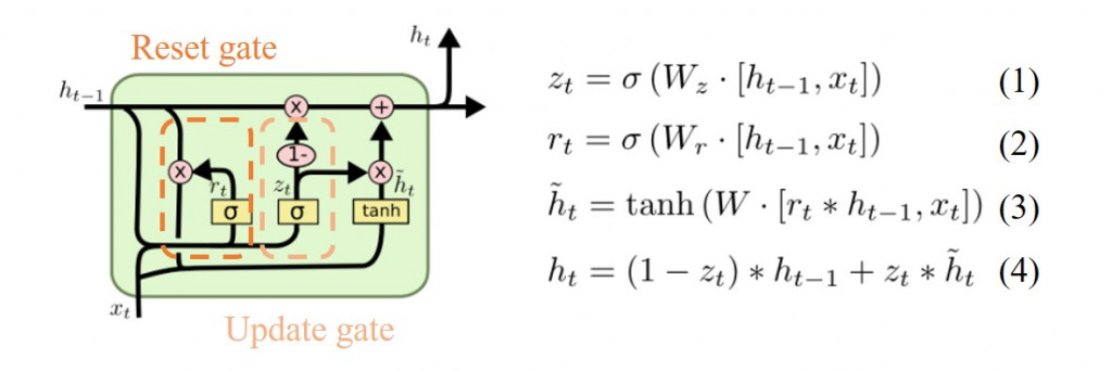

第一條公式為計算更新閥(update gate)的值，激活函數為sigmoid function與LSTM的閥門一樣。第二條與第一條相同，不同的是權重的值。第三條計算輸入經過hyperbolic tangent轉換後的數值，目的是將輸入的範圍縮小至1到-1之間。最後一條計算神經元的輸出值，如果為1輸出經過轉換後的輸入值，如果為0輸出前一個神經元的輸出。

程式碼

今天使用的資料與昨天是一樣的，是我之前我爬蟲抓取ETtoday的新聞，新聞類別有寵物、健康以及旅遊。新聞我已經完成部分的前處理，接著建立字典，字典裡的單字為5000個，將取頻率出現最高的前5000個單字作轉換。

from tensorflow.keras.preprocessing.text import Tokenizer
import pandas as pd
max_words = 5000
max_len = 500
tokenizer = Tokenizer(num_words=max_words)  ## 使用的最大詞語數為5000
news = pd.read_excel('ETtoday news_202205.xlsx', engine = 'openpyxl')
tokenizer.fit_on_texts(news['tokenization'])

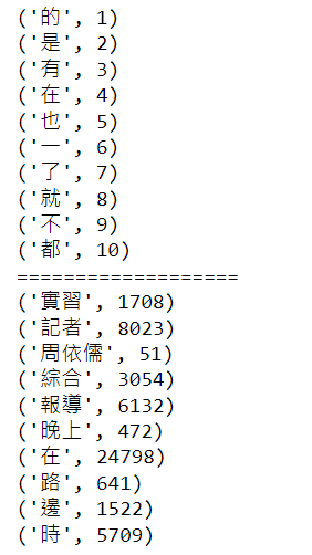
將最常出現的10個單字以及前面10個單字印出

## 使用word_index屬性可以看到每個詞對應的編碼
## 使用word_counts屬性可以看到每個詞對應的頻數
for index,item in enumerate(tokenizer.word_index.items()):
    if index < 10:
        print(item)
    else:
        break
print("===================")  
for index,item in enumerate(tokenizer.word_counts.items()):
    if index < 10:
        print(item)
    else:
        break

將原本新聞類別one-hot encoding轉為數字，並且切割訓練集以及測試集。

from sklearn.preprocessing import OneHotEncoder, LabelEncoder
from sklearn.model_selection import train_test_split
labelencoder = LabelEncoder()
le_y = labelencoder.fit_transform(news['category']).reshape(-1,1)
ohe = OneHotEncoder()
y = ohe.fit_transform(le_y).toarray()
x = news['tokenization']
#Split the data to have 20% validation split
train_x, test_x, train_y, test_y = train_test_split(x, y, test_size=0.2)

將文字轉換為數字，每則新聞最長的長度為500。處理完成後，將資料輸入至GRU模型訓練。

from sklearn import metrics
from tensorflow.keras.models import Model
from tensorflow.keras.layers import GRU, Activation, Dense, Dropout, Input, Embedding
from tensorflow.keras.optimizers import RMSprop
from tensorflow.keras.preprocessing.text import Tokenizer
from tensorflow.keras.preprocessing import sequence

train_seq = tokenizer.texts_to_sequences(train_x)
test_seq = tokenizer.texts_to_sequences(test_x)
## 將每個序列調整相同的長度
train_seq_mat = sequence.pad_sequences(train_seq,maxlen=max_len)
test_seq_mat = sequence.pad_sequences(test_seq,maxlen=max_len)
# print(train_seq_mat.shape, test_seq_mat.shape)
inputs = Input(name='inputs',shape=[max_len])
## Embedding(詞匯表大小,vector長度,每個新聞的詞長)
layer = Embedding(max_words+1,128,input_length=max_len)(inputs)
layer = GRU(128)(layer)
layer = Dense(128,activation="relu",name="FC1")(layer)
layer = Dropout(0.3)(layer)
layer = Dense(3,activation="softmax",name="FC2")(layer)
model = Model(inputs=inputs,outputs=layer)
model.summary()
## multi-classification problem use categorical_crossentropy
model.compile(loss="categorical_crossentropy",optimizer=RMSprop(),metrics=["accuracy"])

model_fit = model.fit(train_seq_mat,train_y,batch_size=128,epochs=10,
                     validation_split=0.2)

檢視訓練的績效

import numpy as np
test_pre = model.predict(test_seq_mat)
## evaluate the performance of prediction
confusion_matrix = metrics.confusion_matrix(np.argmax(test_pre,axis=1),np.argmax(test_y,axis=1))
print("Confusion matrix: \n",confusion_matrix)

scores = model.evaluate(test_seq_mat, test_y, verbose=0)
print("Out-of-sample loss: ", scores[0],"Out-of-sample accuracy:", scores[1])

print(metrics.classification_report(np.argmax(test_pre,axis=1),np.argmax(test_y,axis=1)))

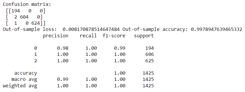
與上一篇LSTM的結果相比，GRU測試集的準確率較低，但是相差不大。每次訓練模型的結果會不一樣，之前我訓練時LSTM的準確率也是99%。

視覺化準確率與損失值的變化

# 繪製歷程圖
import matplotlib.pyplot as plt
def show_train_history(train_history):
    plt.figure(figsize=(6,5))
    plt.plot(train_history.history['accuracy'])
    plt.plot(train_history.history['val_accuracy'])
    plt.xticks([i for i in range(len(train_history.history['accuracy']))])
    plt.title('Train History')
    plt.ylabel('accuracy')
    plt.xlabel('epoch')
    plt.legend(['Train', 'Val'], loc='upper left')
    plt.savefig('Accuracy.png')
    plt.show()

    plt.figure(figsize=(6,5))
    plt.plot(train_history.history['loss'])
    plt.plot(train_history.history['val_loss'])
    plt.xticks([i for i in range(len(train_history.history['loss']))])
    plt.title('Train History')
    plt.ylabel('loss')
    plt.xlabel('epoch')
    plt.legend(['Train', 'Val'], loc='upper left')
    plt.savefig('Loss.png')
    plt.show()
show_train_history(model_fit)

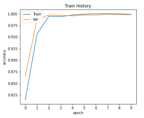
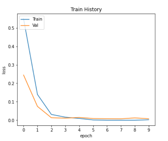
可以從上面兩張圖看出，沒有overfitting的情況。

感謝您的瀏覽，程式碼已上傳Github