[Day15]：想讓訓練更穩定？使用WGAN吧

2023 iThome 鐵人賽

DAY 15

AI & Data

生成式AI到底何方神聖？一窺生程式AI的真面目系列第 15 篇

15th鐵人賽

golucky_sir

2023-09-18 00:29:14

585 瀏覽

分享至

前言

昨天介紹了WGAN的原理，雖然在昨天看到各種公式可能會被嚇到，其中其實也還有許多細節可以介紹。雖然數學公式繁雜，不過建立WGAN模型卻很簡單。接下來就來一步一步建立WGAN吧！

建立WGAN模型

WGAN模型與普通GAN在實作上只有一些差異，分別為：

生成器與判別器使用Wasserstein Loss。
對判別器做權重裁剪。
訓練Label要改成真實資料為-1，生成資料為1。
使用RMSprop優化器，這個優化器使用了動量的概念，使權重更新時能考慮新舊梯度的重要性。
判別器輸出層不使用激活函數，使之成為線性輸出，原因在昨天已經向各位介紹過了喔，因為要讓判別器輸出的是圖片與真實圖片相似的程度，這部分忘記的請去複習一下昨天的文章「與GAN有甚麼不同？」那個部分。

第一步：決定任務類型與要使用的模型

這裡也一樣，使用WGAN做mnist手寫資料集的圖片生成。此外這次的WGAN模型是從DCGAN改來的，而非原始的GAN。

第二步：匯入函式庫

這邊與DCGAN不同的是優化器的使用從Adam變成RMSprop、以及要計算Wasserstein Loss我們需要使用Keras的後端API去計算。
要使用Keras後端必須匯入import tensorflow.keras.backend as K，至於為甚麼叫 ”K” 這我想應該是不成文的規定吧XD，畢竟Github上大家使用都是默認為K。

from tensorflow.keras.datasets import mnist
from tensorflow.keras.layers import Input, Dense, Reshape, Flatten, BatchNormalization, LeakyReLU, Activation, Conv2DTranspose, Conv2D
from tensorflow.keras.models import Model, save_model
from tensorflow.keras.optimizers import RMSprop #RMSprop優化器
import tensorflow.keras.backend as K #Keras後端
import matplotlib.pyplot as plt
import numpy as np
import os

第三步：資料前處理 (Data Preprocessing)

這部分也沒有改變。讓圖片的像素值落在-1~1之間，以符合生成器輸出層的 tanh 激活函數輸出。

def load_data(self):
        (x_train, _), (_, _) = mnist.load_data()  # 底線是未被用到的資料，可忽略
        x_train = (x_train / 127.5)-1  # 正規化
        x_train = x_train.reshape((-1, 28, 28, 1))
        return x_train

第四步：建立生成模型類別

這裡與DCGAN不同的是要新增權重裁剪的上下限(self.clip_value = clip_value)，定義在初始化__init__()方法中。

class WGAN():
    def __init__(self, generator_lr, discriminator_lr, clip_value):
        self.generator_lr = generator_lr
        self.discriminator_lr = discriminator_lr

        self.discriminator = self.build_discriminator()
        self.generator = self.build_generator()
        self.adversarial = self.build_adversarialmodel()
        self.clip_value = clip_value #權重裁剪的上下限

        self.gloss = []
        self.dloss = []
        if not os.path.exists('./result/WGAN/imgs'):# 將訓練過程產生的圖片儲存起來
            os.makedirs('./result/WGAN/imgs')# 如果忘記新增資料夾可以用這個方式建立

第五步：建立模型、定義訓練方法

接著來定義生成器、判別器與對抗模型吧！

生成器：
生成器與DCGAN沒啥差別。

def build_generator(self):
        input_ = Input(shape=(100, ))
        x = Dense(7*7*32)(input_)
        x = BatchNormalization(momentum=0.8)(x)
        x = Activation('relu')(x)
        x = Reshape((7, 7, 32))(x)
        x = Conv2DTranspose(128, kernel_size=4, strides=2, padding='same')(x)
        x = BatchNormalization(momentum=0.8)(x)
        x = Activation('relu')(x)
        x = Conv2DTranspose(256, kernel_size=4, strides=2, padding='same')(x)
        x = BatchNormalization(momentum=0.8)(x)
        x = Activation('relu')(x)
        out = Conv2DTranspose(1, kernel_size=4, strides=1, padding='same', activation='tanh')(x)

        model = Model(inputs=input_, outputs=out, name='Generator')
        model.summary()
        return model

判別器：
判別器要注意輸出層不設定激活函數。

def build_discriminator(self):
        input_ = Input(shape = (28, 28, 1))
        x = Conv2D(256, kernel_size=4, strides=2, padding='same')(input_)
        x = LeakyReLU(alpha=0.2)(x)
        x = Conv2D(128, kernel_size=4, strides=2, padding='same')(x)
        x = LeakyReLU(alpha=0.2)(x)
        x = Conv2D(64, kernel_size=4, strides=1, padding='same')(x)
        x = LeakyReLU(alpha=0.2)(x)
        x = Flatten()(x)
        out = Dense(1)(x) #不設定激活函數

        model = Model(inputs=input_, outputs=out, name='Discriminator')
        dis_optimizer = RMSprop(learning_rate=self.discriminator_lr)
        model.compile(loss=self.wasserstein_loss,
                      optimizer=dis_optimizer,
                      metrics=['accuracy'])
        model.summary()
        return model

Wasserstein Loss：
昨天介紹了一堆公式，但使用了Keras後端來實現Wasserstein Loss其實意外的簡單。K.mean()是計算張量的平均值。

def wasserstein_loss(self, y_true, y_pred): #這個方法的參數是固定的必須要有y_true, y_pred
        return K.mean(y_true * y_pred)

就這樣，沒了XD
不過為甚麼昨天講了一堆公式而今天實作卻變成這樣？原因是因為昨天提到WGAN的判別器會判斷圖片是真實圖片的程度。以往會使用Sigmoid來判斷圖片是真是假的機率，但在WGAN中判別器並沒有輸出函數，也就是線性的輸出，那判別器希望在面對真實圖片與生成圖片的距離盡可能大。要實現這點最好的方式根據以前的實驗就是將生成圖片的label標記為1而真實圖片標記為-1，這些label的輸出將立即帶來損失。圖片的標記方式待會訓練步驟中會定義，這個比較重要需要注意一下！

不過label設定真實圖片為1而生成圖片為-1好像也可以~

對抗模型：
對抗模型也沒有甚麼變動，只有使用RMSprop作為優化器與損失使用自定義的Wasserstein Loss而已。

def build_adversarialmodel(self):
        noise_input = Input(shape=(100, ))
        generator_sample = self.generator(noise_input)
        self.discriminator.trainable = False
        out = self.discriminator(generator_sample)
        model = Model(inputs=noise_input, outputs=out)

        adv_optimizer = RMSprop(learning_rate=self.generator_lr)
        model.compile(loss=self.wasserstein_loss, optimizer=adv_optimizer)
        model.summary()
        return model

訓練步驟：
⚠️這邊要注意一下判別器的權重裁剪的部分喔！以及訓練標籤的設定。
權重裁減的部分流程上來說會

使用迴圈for l in self.discriminator.layers:來讀取每一層的資料。
接著會使用l.get_weights()來取得該層的權重。
再來就是裁剪權重啦，np.clip(w, -self.clip_value, self.clip_value)代表權重 w 如果小於-self.clip_value則 w=-self.clip_value；反之如果權重 w 大於self.clip_value則 w=self.clip_value。另外[元素 for 變數 in 可迭代物件]是Python中生成式的寫法，若不清楚各位可以參考我一年前寫的青澀文章，裡面就有介紹到。
將該層的權重設定為裁剪過後的新權重l.set_weights(weights)。

def train(self, epochs, batch_size=128, sample_interval=50):
        # 準備訓練資料
        x_train = self.load_data()
        # 準備訓練的標籤，分為真實標籤與假標籤，需注意標籤的內容！
        valid = -np.ones((batch_size, 1))
        fake = np.ones((batch_size, 1))
        for epoch in range(epochs):
            # 隨機取一批次的資料用來訓練
            idx = np.random.randint(0, x_train.shape[0], batch_size)
            imgs = x_train[idx]
            # 從常態分佈中採樣一段雜訊
            noise = np.random.normal(0, 1, (batch_size, 100))
            # 生成一批假圖片
            gen_imgs = self.generator.predict(noise)
            # 判別器訓練判斷真假圖片
            d_loss_real = self.discriminator.train_on_batch(imgs, valid)
            d_loss_fake = self.discriminator.train_on_batch(gen_imgs, fake)
            d_loss = 0.5 * np.add(d_loss_real, d_loss_fake)
			# 權重裁剪
            for l in self.discriminator.layers:
                weights = l.get_weights()
                weights = [np.clip(w, -self.clip_value, self.clip_value) for w in weights]
                l.set_weights(weights)
            #儲存鑑別器損失變化 索引值0為損失 索引值1為準確率
            self.dloss.append(d_loss[0])
            # 訓練生成器的生成能力
            noise = np.random.normal(0, 1, (batch_size, 100))
            g_loss = self.adversarial.train_on_batch(noise, valid)
            # 儲存生成器損失變化
            self.gloss.append(g_loss)
            # 將這一步的訓練資訊print出來
            print(f"Epoch:{epoch} [D loss: {d_loss[0]}, acc: {100 * d_loss[1]:.2f}] [G loss: {g_loss}]")
            # 在指定的訓練次數中，隨機生成圖片，將訓練過程的圖片儲存起來
            if epoch % sample_interval == 0:
                self.sample(epoch)
        self.save_data()

定義其他副程式

這邊也沒有變化，唯一需要改變儲存路徑而已：

def save_data(self):
        np.save(file='./result/WGAN/generator_loss.npy',arr=np.array(self.gloss))
        np.save(file='./result/WGAN/discriminator_loss.npy', arr=np.array(self.dloss))
        save_model(model=self.generator,filepath='./result/WGAN/Generator.h5')
        save_model(model=self.discriminator,filepath='./result/WGAN/Discriminator.h5')
        save_model(model=self.adversarial,filepath='./result/WGAN/Adversarial.h5')

以及生成圖片的部分依然不變：

def sample(self, epoch=None, num_images=25, save=True):
        r = int(np.sqrt(num_images))
        noise = np.random.normal(0, 1, (num_images, 100))
        gen_imgs = self.generator.predict(noise)
        gen_imgs = (gen_imgs+1)/2
        fig, axs = plt.subplots(r, r)
        count = 0
        for i in range(r):
            for j in range(r):
                axs[i, j].imshow(gen_imgs[count, :, :, 0], cmap='gray')
                axs[i, j].axis('off')
                count += 1
        if save:
            fig.savefig(f"./result/WGAN/imgs/{epoch}epochs.png")
        else:
            plt.show()
        plt.clos

第六步：開始訓練

接著開始訓練吧，根據一些文獻與實驗，我們將學習率設定0.00005然後裁剪值設定0.01，如下表。

參數	參數值
生成器學習率	0.00005
判別器學習率	0.00005
Batch Size	128
訓練次數	10000
裁剪值(clip value)	0.01

超參數設定各位可以依照自己喜歡調整，並看看實驗結果如何。

if __name__ == '__main__':
    gan = WGAN(generator_lr=0.00005, discriminator_lr=0.00005, clip_value=0.01)
    gan.train(epochs=10000, batch_size=128, sample_interval=200)
    gan.sample(save=False)

第七步：審視訓練結果並改進

損失圖如下，使用WGAN可以比較好的看到生成器的進步狀況，基本上約4000~5000左右生成器就沒什麼進步了：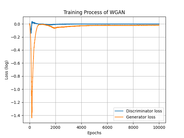

訓練過程跟以往差不多，但很明顯的比較穩定，不像DCGAN花了”億”點點時間調整參數與模型架構，為的就是不要讓訓練失衡。

Epoch=200。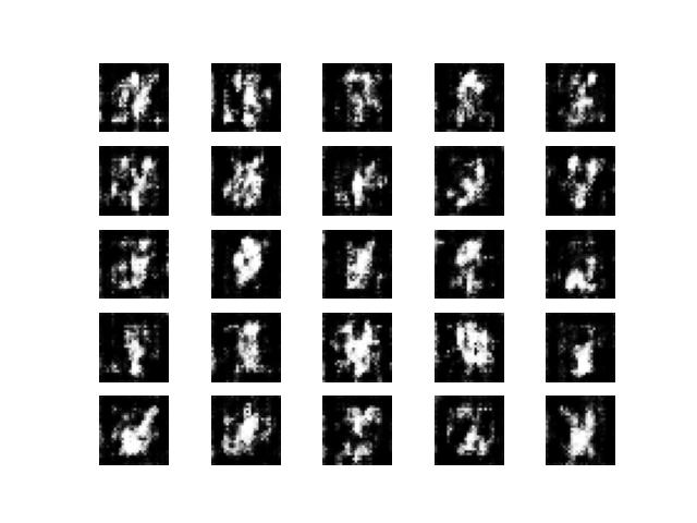

Epoch=2000。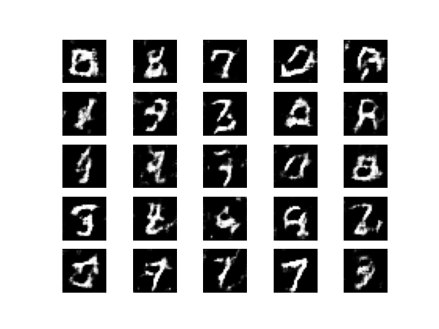

Epoch=5000。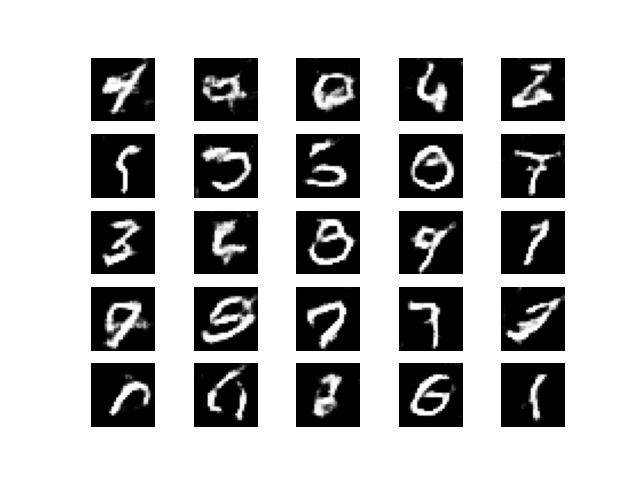

Epoch=10000。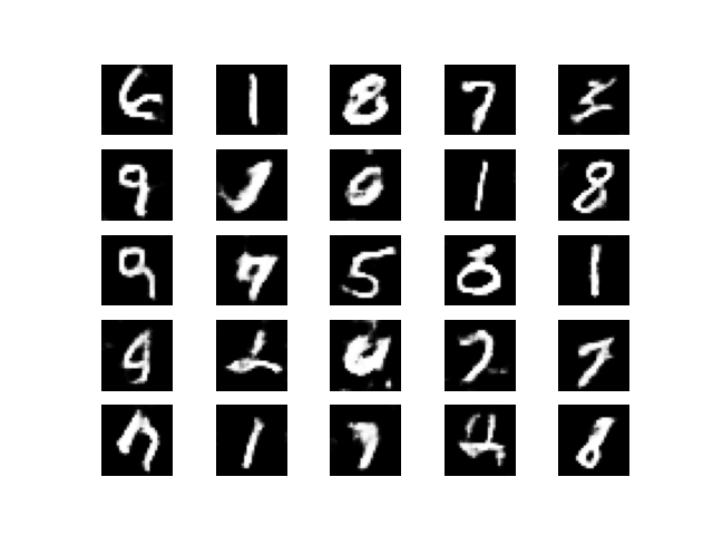

總得來說訓練結果有可能會沒有比DCGAN好，但是WGAN就勝在他訓練穩定且訓練曲線是有意義的。有很多時候不同的GAN訓練不穩定時就會考慮使用WGAN及其變種的方法來改寫網路的目標函數等，所以WGAN對於GAN的發展還是有重大意義的。

最後訓練過程產生的動圖如下：
WGAN

結語

今天帶各位實作了WGAN，雖然數學原理不簡單，但寫成程式後卻意外的簡單呢。不過WGAN在權重裁剪時太暴力了，所以權重有時會處於極端值。對此WGAN-GP解決了這個問題。WGAN-GP主要工作是加入了梯度懲罰，如果梯度的範數偏離其目標範數值，也就是偏離 1 時，WGAN-GP 就會對直接模型進行懲罰，而不是使用梯度裁剪暴力地將梯度值裁剪成上下限值。不過使用這個梯度懲罰的方式會增加計算負擔，使訓練時間變更長，但好處是訓練會比WGAN更穩定。WGAN-GP的具體內容、詳細資訊等各位如果有興趣可以再看看上方超連結喔。

附錄：完整程式

from tensorflow.keras.datasets import mnist
from tensorflow.keras.layers import Input, Dense, Reshape, Flatten, BatchNormalization, LeakyReLU, Activation, Conv2DTranspose, Conv2D
from tensorflow.keras.models import Model, save_model
from tensorflow.keras.optimizers import RMSprop #RMEprop優化器
import tensorflow.keras.backend as K #Keras後端
import matplotlib.pyplot as plt
import numpy as np
import os

class WGAN():
    def __init__(self, generator_lr, discriminator_lr, clip_value):
        self.generator_lr = generator_lr
        self.discriminator_lr = discriminator_lr

        self.discriminator = self.build_discriminator()
        self.generator = self.build_generator()
        self.adversarial = self.build_adversarialmodel()
        self.clip_value = clip_value

        self.gloss = []
        self.dloss = []
        if not os.path.exists('./result/WGAN/imgs'):# 將訓練過程產生的圖片儲存起來
            os.makedirs('./result/WGAN/imgs')# 如果忘記新增資料夾可以用這個方式建立

    def load_data(self):
        (x_train, _), (_, _) = mnist.load_data()  # 底線是未被用到的資料，可忽略
        x_train = (x_train / 127.5)-1  # 正規化
        x_train = x_train.reshape((-1, 28, 28, 1))
        return x_train
    def wasserstein_loss(self, y_true, y_pred):
        return K.mean(y_true * y_pred)
    def build_generator(self):
        input_ = Input(shape=(100, ))
        x = Dense(7*7*32)(input_)
        x = BatchNormalization(momentum=0.8)(x)
        x = Activation('relu')(x)
        x = Reshape((7, 7, 32))(x)
        x = Conv2DTranspose(128, kernel_size=4, strides=2, padding='same')(x)
        x = BatchNormalization(momentum=0.8)(x)
        x = Activation('relu')(x)
        x = Conv2DTranspose(256, kernel_size=4, strides=2, padding='same')(x)
        x = BatchNormalization(momentum=0.8)(x)
        x = Activation('relu')(x)
        out = Conv2DTranspose(1, kernel_size=4, strides=1, padding='same', activation='tanh')(x)

        model = Model(inputs=input_, outputs=out, name='Generator')
        model.summary()
        return model

    def build_discriminator(self):
        input_ = Input(shape = (28, 28, 1))
        x = Conv2D(256, kernel_size=4, strides=2, padding='same')(input_)
        x = LeakyReLU(alpha=0.2)(x)
        x = Conv2D(128, kernel_size=4, strides=2, padding='same')(x)
        x = LeakyReLU(alpha=0.2)(x)
        x = Conv2D(64, kernel_size=4, strides=1, padding='same')(x)
        x = LeakyReLU(alpha=0.2)(x)
        x = Flatten()(x)
        out = Dense(1)(x)

        model = Model(inputs=input_, outputs=out, name='Discriminator')
        dis_optimizer = RMSprop(learning_rate=self.discriminator_lr)
        model.compile(loss=self.wasserstein_loss,
                      optimizer=dis_optimizer,
                      metrics=['accuracy'])
        model.summary()
        return model
    def build_adversarialmodel(self):
        noise_input = Input(shape=(100, ))
        generator_sample = self.generator(noise_input)
        self.discriminator.trainable = False
        out = self.discriminator(generator_sample)
        model = Model(inputs=noise_input, outputs=out)

        adv_optimizer = RMSprop(learning_rate=self.generator_lr)
        model.compile(loss=self.wasserstein_loss, optimizer=adv_optimizer)
        model.summary()
        return model

    def train(self, epochs, batch_size=128, sample_interval=50):
        # 準備訓練資料
        x_train = self.load_data()
        # 準備訓練的標籤，分為真實標籤與假標籤，需注意標籤的內容！
        valid = -np.ones((batch_size, 1))
        fake = np.ones((batch_size, 1))
        for epoch in range(epochs):
            # 隨機取一批次的資料用來訓練
            idx = np.random.randint(0, x_train.shape[0], batch_size)
            imgs = x_train[idx]
            # 從常態分佈中採樣一段雜訊
            noise = np.random.normal(0, 1, (batch_size, 100))
            # 生成一批假圖片
            gen_imgs = self.generator.predict(noise)
            # 判別器訓練判斷真假圖片
            d_loss_real = self.discriminator.train_on_batch(imgs, valid)
            d_loss_fake = self.discriminator.train_on_batch(gen_imgs, fake)
            d_loss = 0.5 * np.add(d_loss_real, d_loss_fake)
			# 權重裁剪
            for l in self.discriminator.layers:
                weights = l.get_weights()
                weights = [np.clip(w, -self.clip_value, self.clip_value) for w in weights]
                l.set_weights(weights)
            #儲存鑑別器損失變化 索引值0為損失 索引值1為準確率
            self.dloss.append(d_loss[0])
            # 訓練生成器的生成能力
            noise = np.random.normal(0, 1, (batch_size, 100))
            g_loss = self.adversarial.train_on_batch(noise, valid)
            # 儲存生成器損失變化
            self.gloss.append(g_loss)
            # 將這一步的訓練資訊print出來
            print(f"Epoch:{epoch} [D loss: {d_loss[0]}, acc: {100 * d_loss[1]:.2f}] [G loss: {g_loss}]")
            # 在指定的訓練次數中，隨機生成圖片，將訓練過程的圖片儲存起來
            if epoch % sample_interval == 0:
                self.sample(epoch)
        self.save_data()
    def save_data(self):
        np.save(file='./result/WGAN/generator_loss.npy',arr=np.array(self.gloss))
        np.save(file='./result/WGAN/discriminator_loss.npy', arr=np.array(self.dloss))
        save_model(model=self.generator,filepath='./result/WGAN/Generator.h5')
        save_model(model=self.discriminator,filepath='./result/WGAN/Discriminator.h5')
        save_model(model=self.adversarial,filepath='./result/WGAN/Adversarial.h5')

    def sample(self, epoch=None, num_images=25, save=True):
        r = int(np.sqrt(num_images))
        noise = np.random.normal(0, 1, (num_images, 100))
        gen_imgs = self.generator.predict(noise)
        gen_imgs = (gen_imgs+1)/2
        fig, axs = plt.subplots(r, r)
        count = 0
        for i in range(r):
            for j in range(r):
                axs[i, j].imshow(gen_imgs[count, :, :, 0], cmap='gray')
                axs[i, j].axis('off')
                count += 1
        if save:
            fig.savefig(f"./result/WGAN/imgs/{epoch}epochs.png")
        else:
            plt.show()
        plt.close()

if __name__ == '__main__':
    gan = WGAN(generator_lr=0.00005,discriminator_lr=0.00005, clip_value=0.01)
    gan.train(epochs=10000, batch_size=128, sample_interval=200)
    gan.sample(save=False)