前言

歷經了前兩天的數學轟炸，希望各位有藉此更加了解擴散模型的原理，今天我們就要來實作DDIM啦，這次使用的程式碼是由Keras 官網上改寫而來的，不過資料集的使用與KID指標的設定都是直接拿現成的，各位可以再根據需求去訓練自己的資料集喔！

建立DDIM模型

這邊一樣使用之前介紹的SOP建立模型，不過每一步的細節都會變多，因為擴散模型除了訓練神經網路以外還要根據公式進行過散與逆向過散，所以程式碼會變得相當長。

第一步：決定任務類型與要使用的模型

這次和官網一樣使用oxford_flowers102資料集，這個資料集包含常見的102種花朵，共有超過10000張圖片被用於訓練！我們要使用DDIM模型去生成這些資料集的圖片。

第二步：匯入函式庫

接著要匯入函式庫，這次用的函式庫相當多，不過我會對一些沒出現過的函式庫進行介紹~

• tfds是可以讓各位載入更多來自官網整理好的資料集，各位可以看看還有甚麼資料集能用，官網對於各類型的任務都有提供相應的資料集使用，非常完整。
• 在DDIM中我們會使用swish激活函數，這個函數在第13天有提到，他是將輸入x乘上sigmoid(x)的結果，長得像ReLU，根據實驗在DDIM中他通常會比一般使用ReLU還好。
• AdamW是Adam的變種，他將權重衰減的部分從函數中拿出來直接加在權重更新步驟上，這樣可以減少計算量，未來我們也會定義AdamW的權重衰減率。
• 為了計算KID，我們會使用InceptionV3模型，這個模型和KID我會在之後詳細介紹。
• 最後就是我們會定義一個Callback，因為是自定義的Callback，所以要使用LambdaCallback。

import math, os
import numpy as np
import matplotlib.pyplot as plt
import tensorflow as tf
import tensorflow_datasets as tfds
from tensorflow.keras.layers import Lambda, GlobalAveragePooling2D, Conv2D, BatchNormalization, Add, AveragePooling2D, UpSampling2D, Concatenate, Input
from keras.layers import Normalization, Rescaling, Resizing
from tensorflow.keras.activations import swish 
from tensorflow.keras.metrics import Metric, Mean
from tensorflow.keras.models import Sequential, Model, save_model, load_model, clone_model
from tensorflow_addons.optimizers import AdamW
from tensorflow.keras.applications.inception_v3 import preprocess_input
from tensorflow.keras.applications import InceptionV3
from tensorflow.keras.callbacks import LambdaCallback
from tensorflow.keras.losses import mean_absolute_error

第三步：資料前處理 (Data Preprocessing)

這次的資料前處理也是拿TensorFlow現成的程式進行資料處理，因為為了運算效率與訓練順利，程式碼的作者對此做了許多處理。這邊就來向各位解釋程式碼的原理。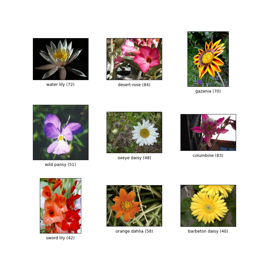

資料集的圖片，使用下列程式碼生成，可以看到圖片長寬不完全相同，這部分需要再做處理：

import tensorflow_datasets as tfds
ds, ds_info = tfds.load('oxford_flowers102', split='train[:80%]+validation[:80%]+test[:80%]', with_info=True)
fig = tfds.show_examples(ds, ds_info)

匯入資料集主要是使用prepare_dataset()方法，在此方法內會有幾個步驟要用來處理資料：

1. 使用tfas.load()來將資料載入進來，並透過split字串來拆分訓練資料。split字串是tfds中特有的設定方式，用於將資料拆成訓練集、驗證集跟測試集。
2. 使用.map()方法，這個方法會將剛剛載入的資料集，對於所有資料都做preprocess_image方法，讓資料集能夠全部變成64x64的大小，並且將像素值正規化到0~1之間。在呼叫函數時使用lambda匿名函數，這樣可以方便傳遞參數。在preprocess_image()中，作者使用tf.image.crop_to_bounding_box將圖片擷取中心部分，因為資料集並不是每張圖片長寬都一樣，所以直接從中心裁剪64x64大小的圖片就可以保證每張圖片的大小相同。
3. 使用.cache()方法將資料集儲存在內存，這樣子在下個epoch中就可以快速讀取資料了！
4. 接著使用.repeat()方法將資料集變成5倍的量，據作者所述在KID計算中，因為KID是嘈雜且計算密集的，所以作者希望在多次迭代之後進行評估，將資料重複5次，這樣訓練一個epoch相當於訓練迭代了5次資料集。
5. 因為重複資料五次，所以要再使用.shuffle()方法將資料集全部再打亂一次。
6. 接著就是將資料使用.batch()拆分成多個批次，用於訓練的drop_remainder=True代表如果最後有剩的資料不足以湊成一批次的話則將那些剩的資料全部丟棄。
7. 最後就是使用.prefetch()來
8. 最後就是使用.prefetch()來設定模型訓練時就預先讀去下次的資料，這樣子在下次訓練時就可以直接調用資料。buffer_size代表要讀取的元素數量，如果設定tf.data.AUTOTUNE參數則會根據可用的CPU動態決定讀去數量。

介紹完了之後真的不禁要感嘆為了加速DDIM訓練，作者真的費盡了心思來處理資料。

def preprocess_image(data, image_size):
    # 建立資料集、將資料裁減中心的區塊、正規化、調整長寬
    height = tf.shape(data["image"])[0]
    width = tf.shape(data["image"])[1]
    crop_size = tf.minimum(height, width)
    image = tf.image.crop_to_bounding_box(data["image"],
        (height - crop_size)//2, (width - crop_size)//2,
        crop_size, crop_size)

    image = tf.image.resize(image, size=[image_size, image_size], antialias=True)
    return tf.clip_by_value(image / 255.0, 0.0, 1.0)

def prepare_dataset(split, batch_size, image_size):
    # 資料增強方法，這一套都是tf寫好的，我認為直接使用即可
    # 若想用其他tf資料集的話可以看看tfds.load()方法中有甚麼dataset可以使用
    return (
        tfds.load(dataset_name, split=split, shuffle_files=True)# 將資料集匯入、拆成訓練 & 驗證 & 測試資料、並隨機打亂。
        .map(lambda data: preprocess_image(data, image_size=image_size), num_parallel_calls=tf.data.AUTOTUNE)# 將preprocess_image方法應用於資料集內所有資料。
        .cache()# 可以把資料集存在內存，以便下個epoch可以快速讀取。
        .repeat(5)# 將資料重複五次
        .shuffle(10 * batch_size)# 再隨機打亂。
        .batch(batch_size, drop_remainder=True)# 將資料集分成指定的批次大小，並將最後剩下湊不出一批次的資料丟棄。
        .prefetch(buffer_size=tf.data.AUTOTUNE))# 在訓練模型時就先讀取的資料，在之後訓練時就可以立即提供。

第四步：建立生成模型類別

接著就是建立DDIM類別啦，作者將這個模型繼承Model類別，使這個模型可以被編譯，且編譯方法可以自定義編譯的內容。

class DiffusionModel(Model):
    def __init__(self, image_size, block_depth, batch_size):
        super().__init__()
        if not os.path.exists('./result/DDIM/imgs'):
            os.makedirs('./result/DDIM/imgs')
        self.batch_size = batch_size
        self.image_size = image_size
        self.normalizer = Normalization()
        self.network = self.get_network(block_depth)
        self.pred_network = clone_model(self.network)

第五步：建立模型、定義訓練方法

這步驟相當複雜，因為有很多東東要建立，不過別擔心，我們一步一步來，先來建立U-Net吧。

U-Net：在Pix2Pix中我們也曾建立過U-Net，這個網路就是在學習預測噪音的。但是在DDIM中的U-Net每層都是多個殘差組合而成的，而且還要建立擴散時間的輸入，所以相較Pix2Pix會比較麻煩。建立神經網路的程式碼如下，以下將解釋一下程式碼中各部分在幹嘛。

1. 首先sinusoidal_embedding()是將擴散時間t輸入並嵌入至神經網路中，要注意的是這個嵌入層與一般的Embedding不同，他使用了一些算法來將擴散時間編碼成一段向量。具體來說首先tf.linspace(tf.math.log(embedding_min_frequency), tf.math.log(1000.0), 16))，他一共會生成起始值是0 (tf.math.log(1.0)=0)到中止值為3 (tf.math.log(1000.0)=3)的值，並根據起始值與中止值生成16個數字的等差數列，數列中的值都是均勻間隔的，這個數列記為 (frequencies )。接著就是計算 跟 ，此時兩個向量都是16的長度，所以會合併成32的長度即為潛入的向量，不過在輸入時會整理成(batch, 1, 1, 1)的shape，所以最後輸入其實shape是 (batch, 1, 1, 32)，這個長度就可以跟第一層卷積合併了！
2. 輸入的部分都處理好就正式來建立殘差的U-Net了，官方使用了閉包的技巧，不過閉包比較抽象，所以這邊以一般的副成是建立為主，首先建立殘差ResidualBlock()，這裡面會包含一個批次正規化BN層、兩個卷積層，其中第一個卷積層使用swish激活函數做輸出，最後再將輸入內容與輸出內容相加起來作為最後的輸出。
3. 每個下採樣DownBlock()與上採樣UpBlock()都是使用兩個殘差做為架構，最後再加一層平均池化層。接著skips會將這層下採樣層存起來，因為等等上採樣層會建立跳接，所以就先存成一個list。
4. 接著上採樣層會先做一次上採樣使輸入大小變為兩倍 ((batch, w, h, u)→(batch, 2w, 2h, u))，再接受來自上個上採樣層與對應的下採樣層的連接，skips.pop()代表將skips中的最後一個元素刪除並回傳最後一個元素，用這個方式也可以建立跳接。接著建立兩個殘差區塊之後再輸出。
5. 最後就是完整建立U-Net了，首先擴散時間輸入並編碼，接著雜訊輸入層經過一個卷積後將兩個輸入合併再輸入至3個下採樣，接著2個殘差塊作為中間層，再接著3個上採樣，最後再經過一個卷積就大功告成了。

為了使各位能更理解skip的功用這邊做了一張圖，希望能幫助各位理解。如果圖畫的不好我很抱歉，本人極度缺乏美術細胞TT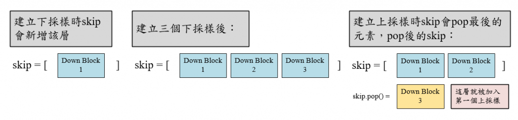

def get_network(self, block_depth):
        def sinusoidal_embedding(x):
            # 將輸入的擴散時間編碼嵌入到模型中
            embedding_min_frequency = 1.0
            frequencies = tf.exp(tf.linspace(tf.math.log(embedding_min_frequency), tf.math.log(1000.0), 16))
            angular_speeds = 2.0 * math.pi * frequencies
            embeddings = tf.concat([tf.sin(angular_speeds * x), tf.cos(angular_speeds * x)], axis=3)
            return embeddings

        def ResidualBlock(x, unit):
            # 殘差層，根據官網址只用兩層CNN組合
            input_unit = x.shape[3]
            if input_unit == unit:
                residual = x
            else:
                residual = Conv2D(unit, kernel_size=1)(x)
            x = BatchNormalization(center=False, scale=False)(x)
            x = Conv2D(unit, kernel_size=3, padding="same", activation=swish)(x)
            x = Conv2D(unit, kernel_size=3, padding="same")(x)
            x = Add()([x, residual])
            return x

        def DownBlock(x, unit, block_depth):
            # 下採樣區塊
            x, skips = x
            for _ in range(block_depth):
                x = ResidualBlock(x, unit)
                skips.append(x)
            x = AveragePooling2D(pool_size=2)(x)
            return x

        def UpBlock(x, unit, block_depth):
            # 上採樣區塊
            x, skips = x
            x = UpSampling2D(size=2, interpolation="bilinear")(x)
            for _ in range(block_depth):
                x = Concatenate()([x, skips.pop()])
                x = ResidualBlock(x, unit)
            return x

        noisy_images = Input(shape=(self.image_size, self.image_size, 3))
        noise_variances = Input(shape=(1, 1, 1))
        e = Lambda(sinusoidal_embedding)(noise_variances)
        e = UpSampling2D(size=self.image_size, interpolation="nearest")(e)
        x = Conv2D(32, kernel_size=1)(noisy_images)  # 第一層卷積
        x = Concatenate()([x, e])
        skips = []
        x = DownBlock([x, skips], 32, block_depth)
        x = DownBlock([x, skips], 64, block_depth)
        x = DownBlock([x, skips], 96, block_depth)
        x = ResidualBlock(x, 128)
        x = ResidualBlock(x, 128)
        x = UpBlock([x, skips], 96, block_depth)
        x = UpBlock([x, skips], 64, block_depth)
        x = UpBlock([x, skips], 32, block_depth)
        x = Conv2D(3, kernel_size=1, kernel_initializer="zeros")(x)
        return Model([noisy_images, noise_variances], x, name="residual_unet")

自定義編譯模型的方法，與評估方法：

自定義編譯模型的方法就是在繼承的類別中覆寫方法，主要是針對損失進行計算。

• noise_loss_tracker：這是針對模型預測的雜訊進行L1損失的計算。
• image_loss_tracker ：這是模型針對一個去噪的圖片進行L1損失的計算。但這個損失並不會用於優化模型，只是看看訓練有沒有進步。
• kid：這不會出現在訓練中，因為這樣訓練時間會變太久了，所以根據官網所述，這個部分被用於訓練完1 epoch時評估模型的時候會計算KID距離。KID的類別定義方法我會附在最底下的附錄。

接著評估方法就是這些指標組合而成，在每個epoch的訓練中都會更新值。可以看到這些值就會被print出來。

def compile(self, **kwargs):
        super().compile(**kwargs)

        self.noise_loss_tracker = Mean(name="n_loss")
        self.image_loss_tracker = Mean(name="i_loss")
        self.kid = KID(name="kid", image_size=self.image_size)

@property
def metrics(self):
    return [self.noise_loss_tracker, self.image_loss_tracker, self.kid]

反正規化方法：denormalize()就提供了這個方法。因為資料在正規化時是使用keras.layers.Normalization() 來正規化，所以就需要根據公式來反正規化，方法是平均self.normalizer.mean加上資料images乘以資料標準差 (變異數 self.normalizer.variance開根號)，最後為了保險起見再將資料的值裁剪使其保持在0~1之間。

def denormalize(self, images):
        # 將正規化後的圖片反轉換回來
        images = self.normalizer.mean + images * self.normalizer.variance**0.5
        return tf.clip_by_value(images, 0.0, 1.0)

擴散方法：來到主軸了，擴散方法他的思想是把一個時間假設為成0~1之間的值，也就是前向擴散過程由t=0開始、t=1結束。在這邊使用了三角函數，將0~1的值變成角度。這邊用了arccos(x)也就是cos的反函數來定義擴散時間的角度最大值與最小值，接著計算當下的擴散時間diffusion_times變成角度的位置，再計算這個擴散時間角度的cos與sin，分別為原始圖片的比例signal_rates與加噪音的程度noise_rates。

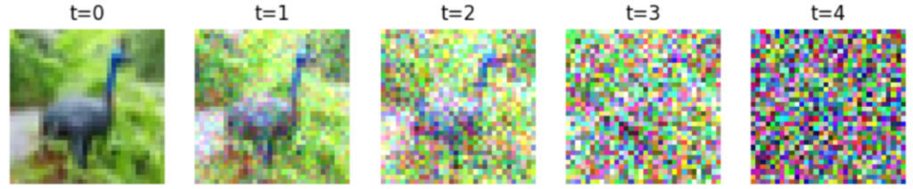
加噪音的方式為：signal_rates * images + noise_rates * noises，images 就是原始圖片，noises就是雜訊。此為方程1，如下。

加噪音後的圖片範例如下圖。可以看到圖片逐漸被加噪音，最後變成完完全全的雜訊，時間 t 只是示意。原始圖片是cifar-10資料集的第7張圖片。加噪音程式如下，這段程式是另外開空白檔案寫的。

from tensorflow.keras.datasets.cifar10 import load_data
import matplotlib.pyplot as plt
import numpy as np
(train_x, train_y), (test_x, test_y) = load_data()
train_x = train_x[6]/255 #可以隨便找一張照片玩玩看
t = np.array([0.999,0.7,0.3,0.001]).reshape((4,1,1,1)) #擴散時間，由左往右是清楚到雜訊
noise_rates, signal_rates = diffusion_schedule(t)
noises = np.random.random(size=(4,32,32,3))
noisy_images = (signal_rates * train_x + noise_rates * noises)
plt.figure(figsize=(10, 4))
plt.subplot(1, 5, 1)
plt.title('t=0')
plt.imshow(train_x)
plt.axis("off")
for row in range(1,5):
    plt.subplot(1, 5, row + 1)
    plt.title(f't={row}')
    plt.imshow(noisy_images[row-1])
    plt.axis("off")
plt.show()

因為cifar-10比較好匯入所以使用這個，至於第7張照片只是我隨便按鍵盤按一個數字而已XD。

加噪音的程度對應到了論文的 ，與另一個原始圖片的比例 ，圖片會透過加噪音的程度去加噪。而且論文中 與 的平方和等於1，cos與sin的平方和也等於1，使用這個方法可以完美達成條件，非常天才。

這個天才辦法根據文章說，此餘弦時間表用於擴散模型出自於這篇文章，他有許多特點，在幾何中也很好解釋。

def diffusion_schedule(self, diffusion_times):
        # 將擴散時間使用反三角函數轉換成介於min_signal_rate ~ max_signal_rate之間的數
        start_angle = tf.acos(max_signal_rate)
        end_angle = tf.acos(min_signal_rate)
        diffusion_angles = start_angle + diffusion_times * (end_angle - start_angle)
        # 這兩個對應到論文中出現的變數，他們的平方和等於1，與論文設定一致。
        signal_rates = tf.cos(diffusion_angles) # α開根號
        noise_rates = tf.sin(diffusion_angles) # (1-α)開根號
        return noise_rates, signal_rates

去噪與逆向擴散：這邊需要提醒一下各位擴散模型的任務就是學會前向擴散過程中加雜訊的分布，接著用於逆向擴散，逆向擴散就是經過很多次去噪而成的。在這邊要定義去噪方式與逆向擴散方式。

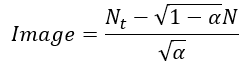
預測的雜訊會經過神經網路計算，接著會將雜訊圖片減去 (noise_rates)乘上預測的雜訊再除以 (signal_rates)，也就是將方程1反過來計算。

逆向擴散就是從從一張隨機雜訊開始，接著一步一步慢慢去噪還原圖片。經過多次去噪還原Image，Image就會逐漸變回原始圖片了！具體來說逆向擴散會輸入一張初始雜訊(initial_noise)，將這個雜訊作為輸入(noisy_images, Nt)，然後計算擴散時間的 與 (noise_rates, signal_rates = self.diffusion_schedule(diffusion_times))，接著預測雜訊分布N再去噪(pred_noises, pred_images = self.denoise(noisy_images, noise_rates, signal_rates, training=False))接著就是更新擴散時間與進行下一次逆向擴散的部分。

def denoise(self, noisy_images, noise_rates, signal_rates, training):
        # 使用類神經網路預測去噪的雜訊、並且去噪
        if training:
            network = self.network
        else:
            network = self.pred_network
        pred_noises = network([noisy_images, noise_rates**2], training=training)
        pred_images = (noisy_images - noise_rates * pred_noises) / signal_rates
        return pred_noises, pred_images

def reverse_diffusion(self, initial_noise, diffusion_steps):
    # 逆擴散過程，採樣一個雜訊
    num_images = initial_noise.shape[0]
    step_size = 1.0 / diffusion_steps
    next_noisy_images = initial_noise
    # 接著一步一步去噪
    for step in range(diffusion_steps):
        noisy_images = next_noisy_images
        diffusion_times = tf.ones((num_images, 1, 1, 1)) - step * step_size
        noise_rates, signal_rates = self.diffusion_schedule(diffusion_times)
        pred_noises, pred_images = self.denoise(noisy_images, noise_rates, signal_rates, training=False)
        next_diffusion_times = diffusion_times - step_size
        next_noise_rates, next_signal_rates = self.diffusion_schedule(next_diffusion_times)
        next_noisy_images = (next_signal_rates * pred_images + next_noise_rates * pred_noises)
    return pred_images

接著生成圖片的方法就是定義雜訊→逆向擴散→反正規化→回傳結果而已。程式碼如下：

def generate(self, num_images, diffusion_steps):
        # 生成圖片，也就是先採樣一個雜訊，接著逆向擴散，最後再逆正規化回來
        initial_noise = tf.random.normal(shape=(num_images, self.image_size, self.image_size, 3))
        generated_images = self.reverse_diffusion(initial_noise, diffusion_steps)
        generated_images = self.denormalize(generated_images)
        return generated_images

訓練方法：接著來定義訓練方法，訓練方法train_step與測試方法test_step都是繼承自Model類別中的方法，裡面做的事情差不多，只是訓練方法會計算梯度、更新權重；測試方法則會評估模型生成的圖片之KID。基本上訓練方式就與類神經訓練差不多，只是要準備雜訊圖片，與去噪的部分而已，詳細說明於底下程式碼。

def train_step(self, images):
        # 繼承Model類別時要定義的方法，也就是每次訓練步驟要幹嘛
        images = self.normalizer(images, training=True)
        noises = tf.random.normal(shape=(self.batch_size, self.image_size, self.image_size, 3))

        # 隨機採樣擴散時間t，再轉換成(1-α)開根號 & α開根號，再根據這個加權添加噪音
        diffusion_times = tf.random.uniform(shape=(self.batch_size, 1, 1, 1), minval=0.0, maxval=1.0)
        noise_rates, signal_rates = self.diffusion_schedule(diffusion_times)
        noisy_images = signal_rates * images + noise_rates * noises

        # 實際訓練神經網路會預測雜訊、逆向擴散成上一個擴散時間的加雜訊圖片，再計算損失
        with tf.GradientTape() as tape:
            pred_noises, pred_images = self.denoise(noisy_images, noise_rates, signal_rates, training=True)
            noise_loss = self.loss(noises, pred_noises)# 實際訓練是要找出雜訊的分布，所以只會使用這個
            image_loss = self.loss(images, pred_images)# 這個是要用於評估的
        # 計算梯度並優化權重，再更新損失訊息
        gradients = tape.gradient(noise_loss, self.network.trainable_weights)
        self.optimizer.apply_gradients(zip(gradients, self.network.trainable_weights))
        self.noise_loss_tracker.update_state(noise_loss)
        self.image_loss_tracker.update_state(image_loss)

        # 把用於預測的網路權重也更新
        for weight, ema_weight in zip(self.network.weights, self.pred_network.weights):
            ema_weight.assign(0.999*ema_weight + 0.001*weight)

        return {m.name: m.result() for m in self.metrics[:-1]}

def test_step(self, images):
    # 測試訓練的部分，此時會評估該次epoch訓練下的模型，其生成圖片的KID結果，與原本定義的損失誤差
    images = self.normalizer(images, training=False)
    noises = tf.random.normal(shape=(self.batch_size, self.image_size, self.image_size, 3))

    diffusion_times = tf.random.uniform(shape=(self.batch_size, 1, 1, 1), minval=0.0, maxval=1.0)
    noise_rates, signal_rates = self.diffusion_schedule(diffusion_times)
    noisy_images = signal_rates * images + noise_rates * noises

    pred_noises, pred_images = self.denoise(noisy_images, noise_rates, signal_rates, training=False)

    noise_loss = self.loss(noises, pred_noises)
    image_loss = self.loss(images, pred_images)

    self.image_loss_tracker.update_state(image_loss)
    self.noise_loss_tracker.update_state(noise_loss)

    images = self.denormalize(images)
    generated_images = self.generate(num_images=self.batch_size, diffusion_steps=kid_diffusion_steps)
    self.kid.update_state(images, generated_images) # 計算生成圖片之KID

    return {m.name: m.result() for m in self.metrics}

定義其他副程式

終於來到最後一步了，這一步就是整理將生成圖片儲存起來而已，以及儲存訓練的損失變化。

def sample(self, epoch=None, logs=None, num_images=9, save=True):
        r = int(np.sqrt(num_images))
        generated_images = self.generate(num_images=r * r, diffusion_steps=plot_diffusion_steps)
        plt.figure(figsize=(18, 18))
        fig, axs = plt.subplots(r, r)
        count = 0
        for i in range(r):
            for j in range(r):
                axs[i, j].imshow(generated_images[count])
                axs[i, j].axis('off')
                count += 1
        plt.tight_layout()
        if save:
            plt.savefig(f"./result/DDIM/imgs/{epoch}epochs.png")
        else:
            plt.show()

損失的部分就是使用model的history物件，他可以儲存模型在訓練過程中產生的損失以及評估方法的結果。這部分就是將他畫出來以利於後續的分析，並儲存每個損失。

def save_loss(self):
        plt.figure(figsize=(8, 6))
        plt.title('Training Loss',fontsize=20)
        plt.xlabel('Epochs',fontsize=17)
        plt.ylabel('Loss',fontsize=17)
        for key in self.history.history:
            plt.plot(self.history.history[key], label=key)
        plt.legend(loc='upper right')
        plt.grid(True)
        plt.savefig(f'./result/DDIM/loss.png')
        for key in self.history.history:
            np.save(arr=self.history.history[key], file=f'./result/DDIM/{key}.npy')

第六步：開始訓練

接著就是開始訓練啦，我們定義了許多參數，其中有一些部分可以對照程式碼的註解：

• kid_image_size代表要使用多少解析度的圖片來評估KID、kid_diffusion_steps也是在使用KID評估時要用幾次去噪來還原圖片，這邊的值設定這樣比較少都是因為要讓訓練快一點。
• 建立資料集並拆分：就是使用文章上面介紹的資料前處理方式處理數據。
• 定義模型與編譯，將訓練資料做標準化：將資料做標準化也是訓練深度學習必備的部分，這裡倒沒什麼值得介紹的。
• 訓練模型：自定義Callback就是定義在每一個epoch結束後(on_epoch_end)，執行方法(model.sample)，生成一批圖片並存起來。
• 訓練完後儲存模型並從訓練完成的模型中再生成圖片，看看訓練完成的模型其生成能力如何。

if __name__=='__main__':
    kid_image_size = 75
    kid_diffusion_steps = 5
    plot_diffusion_steps = 20
    # 建立擴散時間的最大最小值
    min_signal_rate = 0.02
    max_signal_rate = 0.95
    block_depth = 2 # 殘差的層數
    batch_size = 64

    # 建立資料集並拆分
    dataset_name = "oxford_flowers102"
    train_dataset = prepare_dataset("train[:80%]+validation[:80%]+test[:80%]", batch_size=batch_size, image_size=64)
    val_dataset = prepare_dataset("train[80%:]+validation[80%:]+test[80%:]", batch_size=batch_size, image_size=64)
    # 定義模型與編譯，將訓練資料做標準化
    model = DiffusionModel(image_size=64, block_depth=2, batch_size=batch_size)
    model.compile(optimizer=AdamW(learning_rate=0.001, weight_decay=0.0001), loss=mean_absolute_error)
    model.normalizer.adapt(train_dataset)
    # 訓練模型
    model.fit(train_dataset, epochs=50, validation_data=val_dataset,
        callbacks=[LambdaCallback(on_epoch_end=model.sample)]) #使用自定義的Callback
    # 儲存模型
    save_model(model=model.network, filepath='./result/DDIM/DDIM_model.h5')
    # 重新載入模型，並生成圖片。
    network = load_model(filepath='./result/DDIM/DDIM_model.h5')
    model.pred_network = network
    model.sample()
    model.save_loss()

結語

今天介紹的東西太多了XD，所以訓練的結果甚麼的我想要留在明天再向各位介紹。這些程式碼都是出自於官方的範例，只是被我改成我習慣的方式，並介紹給大家。希望各位在今天實作過後能更了解擴散模型的原理以及運作方式。今天說了一堆東東，明天內容應該就會偏少 (絕對不是我想要混一天🤣)，僅僅分享DDIM的訓練成果以及可能會出現的問題而已~

附錄：完整程式 (包括KID方法)

import math, os
import numpy as np
import matplotlib.pyplot as plt
import tensorflow as tf
import tensorflow_datasets as tfds
from tensorflow.keras.layers import Lambda, GlobalAveragePooling2D, Conv2D, BatchNormalization, Add, AveragePooling2D, UpSampling2D, Concatenate, Input
from keras.layers import Normalization, Rescaling, Resizing
from tensorflow.keras.activations import swish
from tensorflow.keras.metrics import Metric, Mean
from tensorflow.keras.models import Sequential, Model, save_model, load_model, clone_model
from tensorflow_addons.optimizers import AdamW
from tensorflow.keras.applications.inception_v3 import preprocess_input
from tensorflow.keras.applications import InceptionV3
from tensorflow.keras.callbacks import LambdaCallback
from tensorflow.keras.losses import mean_absolute_error

def preprocess_image(data, image_size):
    # 建立資料集、將資料裁減中心的區塊、正規化、調整長寬
    height = tf.shape(data["image"])[0]
    width = tf.shape(data["image"])[1]
    crop_size = tf.minimum(height, width)
    image = tf.image.crop_to_bounding_box(data["image"],
        (height - crop_size)//2, (width - crop_size)//2,
        crop_size, crop_size)

    image = tf.image.resize(image, size=[image_size, image_size], antialias=True)
    return tf.clip_by_value(image / 255.0, 0.0, 1.0)

def prepare_dataset(split, batch_size, image_size):
    # 資料增強方法，這一套都是tf寫好的，我認為直接使用即可
    # 若想用其他tf資料集的話可以看看tfds.load()方法中有甚麼dataset可以使用
    return (
        tfds.load(dataset_name, split=split, shuffle_files=True)# 將資料集匯入、拆成訓練 & 驗證 & 測試資料、並隨機打亂。
        .map(lambda data: preprocess_image(data, image_size=image_size), num_parallel_calls=tf.data.AUTOTUNE)# 將preprocess_image方法應用於資料集內所有資料。
        .cache()# 可以把資料集存在內存，以便下個epoch可以快速讀取。
        .repeat(5)# 因為KID是嘈雜且計算密集的，所以作者希望在多次迭代之後進行評估，將資料重複五次，這樣訓練一個epoch相當於訓練迭代了五次資料集。
        .shuffle(10 * batch_size)# 再隨機打亂。
        .batch(batch_size, drop_remainder=True)# 將資料集分成指定的批次大小，並將最後剩下湊不出一批次的資料丟棄。
        .prefetch(buffer_size=tf.data.AUTOTUNE))# 在訓練模型時就先讀取的資料，在之後訓練時就可以立即提供。

class KID(Metric):
    # KID的評估方法就直接使用官網提供的方法，具體之後如何使用這個指標會留到後面再完整介紹
    # 如果是要評估模型效能的話推薦直接使用這段程式碼即可，因為已經繼承Metric類別，在model.compile設定中較不會有衝突
    def __init__(self, name, image_size, **kwargs):
        super().__init__(name=name, **kwargs)
        self.kid_tracker = Mean(name="kid_tracker")

        self.encoder = Sequential([
                Input(shape=(image_size, image_size, 3)),
                Rescaling(255.0),
                Resizing(height=kid_image_size, width=kid_image_size),
                Lambda(preprocess_input),
                InceptionV3(
                    include_top=False,
                    input_shape=(kid_image_size, kid_image_size, 3),
                    weights="imagenet"),
                GlobalAveragePooling2D()], name="inception_encoder")

    def polynomial_kernel(self, features_1, features_2):
        feature_dimensions = tf.cast(tf.shape(features_1)[1], dtype=tf.float32)
        return (features_1 @ tf.transpose(features_2) / feature_dimensions + 1.0) ** 3.0

    def update_state(self, real_images, generated_images, sample_weight=None):
        real_features = self.encoder(real_images, training=False)
        generated_features = self.encoder(generated_images, training=False)

        # compute polynomial kernels using the two sets of features
        kernel_real = self.polynomial_kernel(real_features, real_features)
        kernel_generated = self.polynomial_kernel(
            generated_features, generated_features
        )
        kernel_cross = self.polynomial_kernel(real_features, generated_features)

        # estimate the squared maximum mean discrepancy using the average kernel values
        batch_size = tf.shape(real_features)[0]
        batch_size_f = tf.cast(batch_size, dtype=tf.float32)
        mean_kernel_real = tf.reduce_sum(kernel_real * (1.0 - tf.eye(batch_size))) / (
            batch_size_f * (batch_size_f - 1.0)
        )
        mean_kernel_generated = tf.reduce_sum(
            kernel_generated * (1.0 - tf.eye(batch_size))
        ) / (batch_size_f * (batch_size_f - 1.0))
        mean_kernel_cross = tf.reduce_mean(kernel_cross)
        kid = mean_kernel_real + mean_kernel_generated - 2.0 * mean_kernel_cross

        # update the average KID estimate
        self.kid_tracker.update_state(kid)

    def result(self):
        return self.kid_tracker.result()

    def reset_state(self):
        self.kid_tracker.reset_state()

class DiffusionModel(Model):
    def __init__(self, image_size, block_depth, batch_size):
        super().__init__()
        if not os.path.exists('./result/DDIM/imgs'):
            os.makedirs('./result/DDIM/imgs')
        self.batch_size = batch_size
        self.image_size = image_size
        self.normalizer = Normalization()
        self.network = self.get_network(block_depth)
        self.pred_network = clone_model(self.network)

    def get_network(self, block_depth):
        def sinusoidal_embedding(x):
            # 將輸入的擴散時間編碼嵌入到模型中
            embedding_min_frequency = 1.0
            frequencies = tf.exp(tf.linspace(tf.math.log(embedding_min_frequency), tf.math.log(1000.0), 16))
            angular_speeds = 2.0 * math.pi * frequencies
            embeddings = tf.concat([tf.sin(angular_speeds * x), tf.cos(angular_speeds * x)], axis=3)
            return embeddings

        def ResidualBlock(x, unit):
            # 殘差層，根據官網址只用兩層CNN組合
            input_unit = x.shape[3]
            if input_unit == unit:
                residual = x
            else:
                residual = Conv2D(unit, kernel_size=1)(x)
            x = BatchNormalization(center=False, scale=False)(x)
            x = Conv2D(unit, kernel_size=3, padding="same", activation=swish)(x)
            x = Conv2D(unit, kernel_size=3, padding="same")(x)
            x = Add()([x, residual])
            return x

        def DownBlock(x, unit, block_depth):
            # 下採樣區塊
            x, skips = x
            for _ in range(block_depth):
                x = ResidualBlock(x, unit)
                skips.append(x)
            x = AveragePooling2D(pool_size=2)(x)
            return x

        def UpBlock(x, unit, block_depth):
            # 上採樣區塊
            x, skips = x
            x = UpSampling2D(size=2, interpolation="bilinear")(x)
            for _ in range(block_depth):
                x = Concatenate()([x, skips.pop()])
                x = ResidualBlock(x, unit)
            return x

        noisy_images = Input(shape=(self.image_size, self.image_size, 3))
        noise_variances = Input(shape=(1, 1, 1))
        e = Lambda(sinusoidal_embedding)(noise_variances)
        e = UpSampling2D(size=self.image_size, interpolation="nearest")(e)
        x = Conv2D(32, kernel_size=1)(noisy_images)  # 第一層卷積
        x = Concatenate()([x, e])
        skips = []
        x = DownBlock([x, skips], 32, block_depth)
        x = DownBlock([x, skips], 64, block_depth)
        x = DownBlock([x, skips], 96, block_depth)
        x = ResidualBlock(x, 128)
        x = ResidualBlock(x, 128)
        x = UpBlock([x, skips], 96, block_depth)
        x = UpBlock([x, skips], 64, block_depth)
        x = UpBlock([x, skips], 32, block_depth)
        x = Conv2D(3, kernel_size=1, kernel_initializer="zeros")(x)
        return Model([noisy_images, noise_variances], x, name="residual_unet")

    def compile(self, **kwargs):
        super().compile(**kwargs)

        self.noise_loss_tracker = Mean(name="n_loss")
        self.image_loss_tracker = Mean(name="i_loss")
        self.kid = KID(name="kid", image_size=self.image_size)

    @property
    def metrics(self):
        return [self.noise_loss_tracker, self.image_loss_tracker, self.kid]

    def denormalize(self, images):
        # 將正規化後的圖片反轉換回來
        images = self.normalizer.mean + images * self.normalizer.variance**0.5
        return tf.clip_by_value(images, 0.0, 1.0)

    def diffusion_schedule(self, diffusion_times):
        # 將擴散時間使用三角函數轉換成介於min_signal_rate ~ max_signal_rate之間的數
        start_angle = tf.acos(max_signal_rate)
        end_angle = tf.acos(min_signal_rate)
        diffusion_angles = start_angle + diffusion_times * (end_angle - start_angle)
        # 這兩個對應到論文中出現的變數，他們的平方和等於1，與論文設定一致。
        signal_rates = tf.cos(diffusion_angles) # α開根號
        noise_rates = tf.sin(diffusion_angles) # (1-α)開根號
        return noise_rates, signal_rates

    def denoise(self, noisy_images, noise_rates, signal_rates, training):
        # 使用類神經網路預測去噪的雜訊、並且去噪
        if training:
            network = self.network
        else:
            network = self.pred_network
        pred_noises = network([noisy_images, noise_rates**2], training=training)
        pred_images = (noisy_images - noise_rates * pred_noises) / signal_rates
        return pred_noises, pred_images

    def reverse_diffusion(self, initial_noise, diffusion_steps):
        # 逆擴散過程，採樣一個雜訊
        num_images = initial_noise.shape[0]
        step_size = 1.0 / diffusion_steps
        next_noisy_images = initial_noise #初始雜訊
        # 接著一步一步去噪
        for step in range(diffusion_steps):
            noisy_images = next_noisy_images
            diffusion_times = tf.ones((num_images, 1, 1, 1)) - step * step_size
            noise_rates, signal_rates = self.diffusion_schedule(diffusion_times)
            pred_noises, pred_images = self.denoise(noisy_images, noise_rates, signal_rates, training=False)
            next_diffusion_times = diffusion_times - step_size
            next_noise_rates, next_signal_rates = self.diffusion_schedule(next_diffusion_times)
            next_noisy_images = (next_signal_rates * pred_images + next_noise_rates * pred_noises)
        return pred_images

    def generate(self, num_images, diffusion_steps):
        # 生成圖片，也就是先採樣一個雜訊，接著逆向擴散，最後再逆正規化回來
        initial_noise = tf.random.normal(shape=(num_images, self.image_size, self.image_size, 3))
        generated_images = self.reverse_diffusion(initial_noise, diffusion_steps)
        generated_images = self.denormalize(generated_images)
        return generated_images

    def train_step(self, images):
        # 繼承Model類別時要定義的方法，也就是每次訓練步驟要幹嘛
        images = self.normalizer(images, training=True)
        noises = tf.random.normal(shape=(self.batch_size, self.image_size, self.image_size, 3))

        # 隨機採樣擴散時間t，再轉換成(1-α)開根號 & α開根號，再根據這個加權添加噪音
        diffusion_times = tf.random.uniform(shape=(self.batch_size, 1, 1, 1), minval=0.0, maxval=1.0)
        noise_rates, signal_rates = self.diffusion_schedule(diffusion_times)
        noisy_images = signal_rates * images + noise_rates * noises

        # 實際訓練神經網路會預測雜訊、逆向擴散成上一個擴散時間的加雜訊圖片，再計算損失
        with tf.GradientTape() as tape:
            pred_noises, pred_images = self.denoise(noisy_images, noise_rates, signal_rates, training=True)
            noise_loss = self.loss(noises, pred_noises)# 實際訓練是要找出雜訊的分布，所以只會使用這個
            image_loss = self.loss(images, pred_images)# 這個是要用於評估的
        # 計算梯度並優化權重，再更新損失訊息
        gradients = tape.gradient(noise_loss, self.network.trainable_weights)
        self.optimizer.apply_gradients(zip(gradients, self.network.trainable_weights))
        self.noise_loss_tracker.update_state(noise_loss)
        self.image_loss_tracker.update_state(image_loss)

        # 把用於預測的網路權重也更新
        for weight, ema_weight in zip(self.network.weights, self.pred_network.weights):
            ema_weight.assign(0.999*ema_weight + 0.001*weight)

        return {m.name: m.result() for m in self.metrics[:-1]}

    def test_step(self, images):
        # 測試訓練的部分，此時會評估該次epoch訓練下的模型，其生成圖片的KID結果
        images = self.normalizer(images, training=False)
        noises = tf.random.normal(shape=(self.batch_size, self.image_size, self.image_size, 3))

        diffusion_times = tf.random.uniform(shape=(self.batch_size, 1, 1, 1), minval=0.0, maxval=1.0)
        noise_rates, signal_rates = self.diffusion_schedule(diffusion_times)
        noisy_images = signal_rates * images + noise_rates * noises

        pred_noises, pred_images = self.denoise(noisy_images, noise_rates, signal_rates, training=False)

        noise_loss = self.loss(noises, pred_noises)
        image_loss = self.loss(images, pred_images)

        self.image_loss_tracker.update_state(image_loss)
        self.noise_loss_tracker.update_state(noise_loss)

        images = self.denormalize(images)
        generated_images = self.generate(num_images=self.batch_size, diffusion_steps=kid_diffusion_steps)
        self.kid.update_state(images, generated_images)

        return {m.name: m.result() for m in self.metrics}
    def save_loss(self):
        plt.figure(figsize=(8, 6))
        plt.title('Training Loss',fontsize=20)
        plt.xlabel('Epochs',fontsize=17)
        plt.ylabel('Loss',fontsize=17)
        for key in self.history.history:
            plt.plot(self.history.history[key], label=key)
        plt.legend(loc='upper right')
        plt.grid(True)
        plt.savefig(f'./result/DDIM/loss.png')
        for key in self.history.history:
            np.save(arr=self.history.history[key], file=f'./result/DDIM/{key}.npy')
    def sample(self, epoch=None, logs=None, num_images=9, save=True):
        r = int(np.sqrt(num_images))
        generated_images = self.generate(num_images=r * r, diffusion_steps=plot_diffusion_steps)
        plt.figure(figsize=(18, 18))
        fig, axs = plt.subplots(r, r)
        count = 0
        for i in range(r):
            for j in range(r):
                axs[i, j].imshow(generated_images[count])
                axs[i, j].axis('off')
                count += 1
        plt.tight_layout()
        if save:
            plt.savefig(f"./result/DDIM/imgs/{epoch}epochs.png")
        else:
            plt.show()

if __name__=='__main__':
    kid_image_size = 75
    kid_diffusion_steps = 5
    plot_diffusion_steps = 20
    # 建立擴散時間的最大最小值
    min_signal_rate = 0.02
    max_signal_rate = 0.95
    block_depth = 2 # 殘差的層數
    batch_size = 64

    # 建立資料集並拆分
    dataset_name = "oxford_flowers102"
    train_dataset = prepare_dataset("train[:80%]+validation[:80%]+test[:80%]", batch_size=batch_size, image_size=64)
    val_dataset = prepare_dataset("train[80%:]+validation[80%:]+test[80%:]", batch_size=batch_size, image_size=64)
    # 定義模型與編譯，將訓練資料做標準化
    model = DiffusionModel(image_size=64, block_depth=2, batch_size=batch_size)
    model.compile(optimizer=AdamW(learning_rate=0.001, weight_decay=0.0001), loss=mean_absolute_error)
    model.normalizer.adapt(train_dataset)
    # 訓練模型
    model.fit(train_dataset, epochs=50, validation_data=val_dataset,
        callbacks=[LambdaCallback(on_epoch_end=model.sample)]) #使用自定義的Callback
    # 儲存模型
    save_model(model=model.network, filepath='./result/DDIM/DDIM_model.h5')
    # 重新載入模型，並生成圖片。
    network = load_model(filepath='./result/DDIM/DDIM_model.h5')
    model.pred_network = network
    model.sample()
    model.save_loss()