影像處理大致上可分為7個步驟：
1.擷取影像(acquiring the image):可能從相機來或電子顯微鏡。
2.前置處理(preprocessing):將影像處理程適合接下來步驟的樣子。
3.切割(segmentation):例如擷取車牌號碼
4.表示與描述(representation and description):尋找曲線或corner來辨識車牌數字
5.辨識與解讀(recognition and interpretation):給物體不同標示與意義，例如是那個縣市的車

數位影像的類型有四種：
1.Binary:二元影像非黑即白，每個像素只佔1位元。適合文字、指紋等。
2.Grayscal:灰階影像從0(黑)~255(白)，每個像素8位元。
3.RGB:由紅藍綠調配深淺從0~255，有255的三次方需要用24-bit又稱24位元彩色影像。
4.Indexed:大部分影像都只用到1600萬種可能顏色的一小部分。為了方便儲存及處理於是建立色譜(color map)或調色盤(color palette)。每個像素的值不代表像素的顏色，是代表色譜上對應顏色的索引(index)ex:GIF檔

認識數位影像的儲存格式後，要來學習一下幾個常用的影像處理演算法

Histogram Equalization

Histogram灰階影像的直方圖，可以推論出影像大致上的特性。較暗的影像灰階值聚集在數值低的區域，整體亮的或曝光過度的灰階值聚集在數值高的區域，對比均衡灰階值平均分散於所有範圍。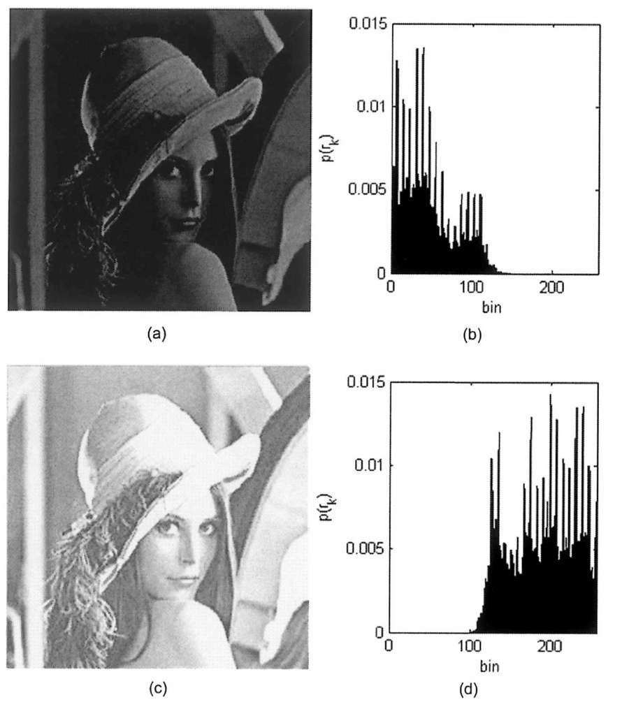

我們從scikit-image的參考網站來測試灰階直方圖等化效果

import matplotlib
import matplotlib.pyplot as plt
import numpy as np

from skimage import data, img_as_float
from skimage import exposure


matplotlib.rcParams['font.size'] = 8


def plot_img_and_hist(image, axes, bins=256):
    """Plot an image along with its histogram and cumulative histogram.

    """
    image = img_as_float(image)
    ax_img, ax_hist = axes
    ax_cdf = ax_hist.twinx()

    # Display image
    ax_img.imshow(image, cmap=plt.cm.gray)
    ax_img.set_axis_off()

    # Display histogram
    ax_hist.hist(image.ravel(), bins=bins, histtype='step', color='black')
    ax_hist.ticklabel_format(axis='y', style='scientific', scilimits=(0, 0))
    ax_hist.set_xlabel('Pixel intensity')
    ax_hist.set_xlim(0, 1)
    ax_hist.set_yticks([])

    # Display cumulative distribution
    img_cdf, bins = exposure.cumulative_distribution(image, bins)
    ax_cdf.plot(bins, img_cdf, 'r')
    ax_cdf.set_yticks([])

    return ax_img, ax_hist, ax_cdf


# Load an example image
img = data.moon()

# Contrast stretching
p2, p98 = np.percentile(img, (2, 98))
img_rescale = exposure.rescale_intensity(img, in_range=(p2, p98))

# Equalization
img_eq = exposure.equalize_hist(img)

# Adaptive Equalization
img_adapteq = exposure.equalize_adapthist(img, clip_limit=0.03)

# Display results
fig = plt.figure(figsize=(8, 5))
axes = np.zeros((2, 4), dtype=np.object)
axes[0, 0] = fig.add_subplot(2, 4, 1)
for i in range(1, 4):
    axes[0, i] = fig.add_subplot(2, 4, 1+i, sharex=axes[0,0], sharey=axes[0,0])
for i in range(0, 4):
    axes[1, i] = fig.add_subplot(2, 4, 5+i)

ax_img, ax_hist, ax_cdf = plot_img_and_hist(img, axes[:, 0])
ax_img.set_title('Low contrast image')

y_min, y_max = ax_hist.get_ylim()
ax_hist.set_ylabel('Number of pixels')
ax_hist.set_yticks(np.linspace(0, y_max, 5))

ax_img, ax_hist, ax_cdf = plot_img_and_hist(img_rescale, axes[:, 1])
ax_img.set_title('Contrast stretching')

ax_img, ax_hist, ax_cdf = plot_img_and_hist(img_eq, axes[:, 2])
ax_img.set_title('Histogram equalization')

ax_img, ax_hist, ax_cdf = plot_img_and_hist(img_adapteq, axes[:, 3])
ax_img.set_title('Adaptive equalization')

ax_cdf.set_ylabel('Fraction of total intensity')
ax_cdf.set_yticks(np.linspace(0, 1, 5))

# prevent overlap of y-axis labels
fig.tight_layout()
plt.show()

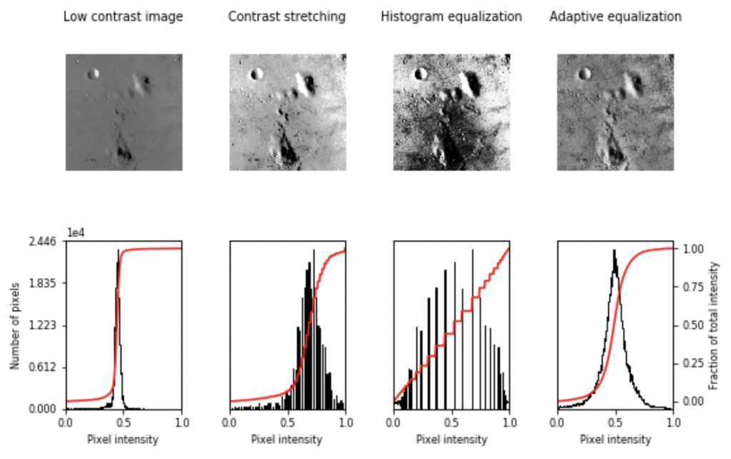
可以發現 Adaptive Equalization(適應性等化)讓圖片的品質更好，有點像高斯分佈。

Neighborhood Processing

鄰域處理針對指定像素周圍鄰近的像素做交互作用，可以花個三分鐘看一下影片就大概了解原理了。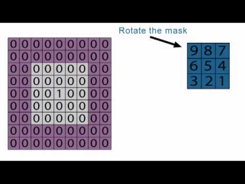

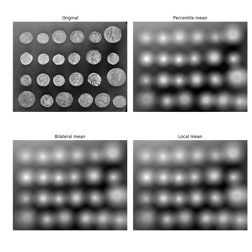
Blur

模糊化的原理可以參考阿州的程式教學，模糊的概念是利用與鄰域的灰階取平均來做到。我們直接使用scikit-image裡面的範例來跑一次，三種不同模糊的演算法在裡面都有解釋。

%matplotlib inline
import matplotlib.pyplot as plt

from skimage import data
from skimage.morphology import disk
from skimage.filters import rank


image = data.coins()
selem = disk(20)

percentile_result = rank.mean_percentile(image, selem=selem, p0=.1, p1=.9)
bilateral_result = rank.mean_bilateral(image, selem=selem, s0=500, s1=500)
normal_result = rank.mean(image, selem=selem)

fig, axes = plt.subplots(nrows=2, ncols=2, figsize=(10, 10),
                         sharex=True, sharey=True)
ax = axes.ravel()

titles = ['Original', 'Percentile mean', 'Bilateral mean', 'Local mean']
imgs = [image, percentile_result, bilateral_result, normal_result]
for n in range(0, len(imgs)):
    ax[n].imshow(imgs[n], cmap=plt.cm.gray)
    ax[n].set_title(titles[n])
    ax[n].axis('off')

plt.tight_layout()
plt.show()

明天再來學習二值化與銳利化和其他常用的演算法～