[魔法陣系列] Recurrent Neural Network（RNN）之術式解析 中介紹了：

• Simple RNN
• LSTM
• GRU

本篇文章要帶各位見習魔法使搭建一個 LSTM 的神經網絡，與 CNN 的實戰系列一樣，採用 Keras 作為實作的工具。

模型任務

預測股票趨勢（上漲/下跌）

資料集

• 訓練集：2012 年 ~ 2016 年的 Google stock price（共 1258 天）
• 測試集：2017 年 1 月的 Google stock price（共 20 天）
• 資料長相：

執行環境版本

Keras 2.1.5
Python 3.6.4

Step 1: 資料前處理

• Load Data：

# Import the libraries
import numpy as np
import matplotlib.pyplot as plt  # for 畫圖用
import pandas as pd

# Import the training set
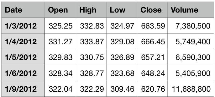
dataset_train = pd.read_csv('Google_Stock_Price_Train.csv')  # 讀取訓練集
training_set = dataset_train.iloc[:, 1:2].values  # 取「Open」欄位值

• 做 Normalization，將資料壓縮在 [0,1] 之間：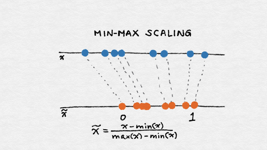
  

圖片來源：《Feature Engineering for Machine Learning》一書

# Feature Scaling
from sklearn.preprocessing import MinMaxScaler

sc = MinMaxScaler(feature_range = (0, 1))
training_set_scaled = sc.fit_transform(training_set)

• 準備進入訓練的資料格式：設定 Timestep
  Timesteps 設為 60 ，代表過去 60 天的資訊，嘗試過數值設置太少，將使 RNN 無法學習。

X_train = []   #預測點的前 60 天的資料
y_train = []   #預測點
for i in range(60, 1258):  # 1258 是訓練集總數
    X_train.append(training_set_scaled[i-60:i, 0])
    y_train.append(training_set_scaled[i, 0])
X_train, y_train = np.array(X_train), np.array(y_train)  # 轉成numpy array的格式，以利輸入 RNN

• Reshape
  因為現在 X_train 是 2-dimension，將它 reshape 成 3-dimension: [stock prices, timesteps, indicators]

X_train = np.reshape(X_train, (X_train.shape[0], X_train.shape[1], 1))

Step 2: 搭建一個 LSTM 魔法陣

• import Keras

# Import the Keras libraries and packages
from keras.models import Sequential
from keras.layers import Dense
from keras.layers import LSTM
from keras.layers import Dropout

# Initialising the RNN
regressor = Sequential()

• 搭建 LSTM layer:
  • units: 神經元的數目
  • 第一層的 LSTM Layer 記得要設定input_shape參數
  • 搭配使用dropout，這裡設為 0.2
  • 由於這邊的第四層 LSTM Layer 即將跟 Ouput Layer 做連接，因此注意這邊的 return_sequences 設為預設值 False （也就是不用寫上 return_sequences）

# Adding the first LSTM layer and some Dropout regularisation
regressor.add(LSTM(units = 50, return_sequences = True, input_shape = (X_train.shape[1], 1)))
regressor.add(Dropout(0.2))

# Adding a second LSTM layer and some Dropout regularisation
regressor.add(LSTM(units = 50, return_sequences = True))
regressor.add(Dropout(0.2))

# Adding a third LSTM layer and some Dropout regularisation
regressor.add(LSTM(units = 50, return_sequences = True))
regressor.add(Dropout(0.2))

# Adding a fourth LSTM layer and some Dropout regularisation
regressor.add(LSTM(units = 50))
regressor.add(Dropout(0.2))

• Ouput Layer: units 設為 1

# Adding the output layer
regressor.add(Dense(units = 1))

• Compiling & Fitting LSTM model
  • optimizer: 選擇 Adam
  • loss: 使用 MSE

# Compiling
regressor.compile(optimizer = 'adam', loss = 'mean_squared_error')

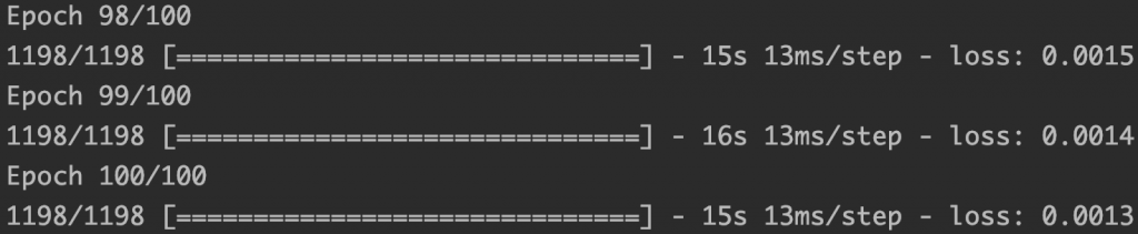
# 進行訓練
regressor.fit(X_train, y_train, epochs = 100, batch_size = 32)

Step 3: 進行預測

• 取測試集中 2017 年的股票資料（真實）

dataset_test = pd.read_csv('Google_Stock_Price_Test.csv')
real_stock_price = dataset_test.iloc[:, 1:2].values

• 取模型所預測的 2017 年股票資料（預測）

dataset_total = pd.concat((dataset_train['Open'], dataset_test['Open']), axis = 0)
inputs = dataset_total[len(dataset_total) - len(dataset_test) - 60:].values
inputs = inputs.reshape(-1,1)
inputs = sc.transform(inputs) # Feature Scaling

X_test = []
for i in range(60, 80):  # timesteps一樣60； 80 = 先前的60天資料+2017年的20天資料
    X_test.append(inputs[i-60:i, 0])
X_test = np.array(X_test)
X_test = np.reshape(X_test, (X_test.shape[0], X_test.shape[1], 1))  # Reshape 成 3-dimension

• 進行預測

predicted_stock_price = regressor.predict(X_test)
predicted_stock_price = sc.inverse_transform(predicted_stock_price)  # to get the original scale

• 視覺化結果

# Visualising the results
plt.plot(real_stock_price, color = 'red', label = 'Real Google Stock Price')  # 紅線表示真實股價
plt.plot(predicted_stock_price, color = 'blue', label = 'Predicted Google Stock Price')  # 藍線表示預測股價
plt.title('Google Stock Price Prediction')
plt.xlabel('Time')
plt.ylabel('Google Stock Price')
plt.legend()
plt.show()

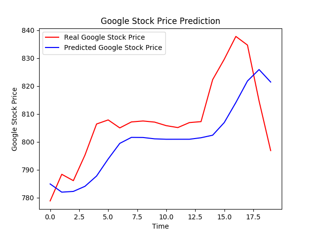
本次模型的任務是預測股票趨勢，由視覺化結果可以看出模型的預測表現，如預測的趨勢雖大致上跟真實股價是一致但預測的較為平滑。