熟悉TensorFlow的第一步就是製作線性回歸（linear regression），此篇也是從First Steps with TensorFlow而來，以Colab網站進行練習。

目標將會學會：

• 學習基本的 TensorFlow 概念
• 在 TensorFlow 中使用 LinearRegressor 類別並預測整個街區的房屋價值中位數
• 使用均方根誤差（RMSE）評估模型預測的準確率
• 修改超參數

線性回歸大概會長成這樣：

（內容稍不齊全，會再修飾一下）

開始

一開始先載入需要的資料庫：

from __future__ import print_function

import math

from IPython import display
from matplotlib import cm
from matplotlib import gridspec
from matplotlib import pyplot as plt
import numpy as np
import pandas as pd
from sklearn import metrics
import tensorflow as tf
from tensorflow.python.data import Dataset

tf.logging.set_verbosity(tf.logging.ERROR)
pd.options.display.max_rows = 10
pd.options.display.float_format = '{:.1f}'.format

接著載入資料。此份是加州的1990年的人口普查資料：

california_housing_dataframe = pd.read_csv("https://download.mlcc.google.cn/mledu-datasets/california_housing_train.csv", sep=",")

在進行之前，先把資料過濾一下，減少發生誤差發生，所以先把資料除以1000。在全體資料減少1000，整體數據縮小，減少部分奇怪資料（髒資料）影響結果。

california_housing_dataframe = california_housing_dataframe.reindex(
    np.random.permutation(california_housing_dataframe.index))
california_housing_dataframe["median_house_value"] /= 1000.0
california_housing_dataframe

檢查數據

在開始使用之前，最好先了解資料。常常看到有人用資料，卻不知道資料的意義，以及資料是否乾淨與否。理論上資料都要是能用的，但是實務上，卻很難達到，所以要先確定資料本身的意義，才能確定我們之後的結果會達到預期。如果一開始就是有問題的資料與欄位，最後結果一定會有所影響。
所以這邊會輸出：樣本數、均質、標準偏差、最大值、最小值、分位數。

california_housing_dataframe.describe()

建立模型特徵列

在本練習中，將會把label設定為median_house_value，也就是我們的目標，並且使用total_rooms當做輸入的特徵。將使用TensorFlow之Estimator API提供的LinearRegressor接口。此API負責處理大量的低級別模型搭建工作，並提供模型訓練、評估、推理等等功能。

而這份數據是程市街區級別，該特徵數據表示鄉對應街區內的房間總數。

首先輸入特徵值：

# Define the input feature: total_rooms.
my_feature = california_housing_dataframe[["total_rooms"]]

# Configure a numeric feature column for total_rooms.
feature_columns = [tf.feature_column.numeric_column("total_rooms")]

訂定目標

# Define the label.
targets = california_housing_dataframe["median_house_value"]

配置 LinearRegressor

# Use gradient descent as the optimizer for training the model.
my_optimizer=tf.train.GradientDescentOptimizer(learning_rate=0.0000001)
my_optimizer = tf.contrib.estimator.clip_gradients_by_norm(my_optimizer, 5.0)

# Configure the linear regression model with our feature columns and optimizer.
# Set a learning rate of 0.0000001 for Gradient Descent.
linear_regressor = tf.estimator.LinearRegressor(
    feature_columns=feature_columns,
    optimizer=my_optimizer
)

定義輸入函數

def my_input_fn(features, targets, batch_size=1, shuffle=True, num_epochs=None):
  
    # Convert pandas data into a dict of np arrays.
    features = {key:np.array(value) for key,value in dict(features).items()}                                           
 
    # Construct a dataset, and configure batching/repeating.
    ds = Dataset.from_tensor_slices((features,targets)) # warning: 2GB limit
    ds = ds.batch(batch_size).repeat(num_epochs)
    
    # Shuffle the data, if specified.
    if shuffle:
      ds = ds.shuffle(buffer_size=10000)
    
    # Return the next batch of data.
    features, labels = ds.make_one_shot_iterator().get_next()
    return features, labels

訓練模型

_ = linear_regressor.train(
    input_fn = lambda:my_input_fn(my_feature, targets),
    steps=100
)

評估模型

# Create an input function for predictions.
# Note: Since we're making just one prediction for each example, we don't 
# need to repeat or shuffle the data here.
prediction_input_fn =lambda: my_input_fn(my_feature, targets, num_epochs=1, shuffle=False)

# Call predict() on the linear_regressor to make predictions.
predictions = linear_regressor.predict(input_fn=prediction_input_fn)

# Format predictions as a NumPy array, so we can calculate error metrics.
predictions = np.array([item['predictions'][0] for item in predictions])

# Print Mean Squared Error and Root Mean Squared Error.
mean_squared_error = metrics.mean_squared_error(predictions, targets)
root_mean_squared_error = math.sqrt(mean_squared_error)
print("Mean Squared Error (on training data): %0.3f" % mean_squared_error)
print("Root Mean Squared Error (on training data): %0.3f" % root_mean_squared_error)

圖表：

sample = california_housing_dataframe.sample(n=300)

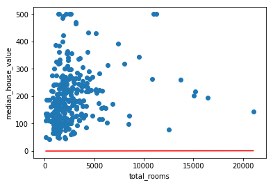
（可以發現誤差很大，紅線根本就是來亂的）

# Get the min and max total_rooms values.
x_0 = sample["total_rooms"].min()
x_1 = sample["total_rooms"].max()

# Retrieve the final weight and bias generated during training.
weight = linear_regressor.get_variable_value('linear/linear_model/total_rooms/weights')[0]
bias = linear_regressor.get_variable_value('linear/linear_model/bias_weights')

# Get the predicted median_house_values for the min and max total_rooms values.
y_0 = weight * x_0 + bias 
y_1 = weight * x_1 + bias

# Plot our regression line from (x_0, y_0) to (x_1, y_1).
plt.plot([x_0, x_1], [y_0, y_1], c='r')

# Label the graph axes.
plt.ylabel("median_house_value")
plt.xlabel("total_rooms")

# Plot a scatter plot from our data sample.
plt.scatter(sample["total_rooms"], sample["median_house_value"])

# Display graph.
plt.show()

調整模型超參數

def train_model(learning_rate, steps, batch_size, input_feature="total_rooms"):
  """Trains a linear regression model of one feature.
  
  Args:
    learning_rate: A `float`, the learning rate.
    steps: A non-zero `int`, the total number of training steps. A training step
      consists of a forward and backward pass using a single batch.
    batch_size: A non-zero `int`, the batch size.
    input_feature: A `string` specifying a column from `california_housing_dataframe`
      to use as input feature.
  """
  
  periods = 10
  steps_per_period = steps / periods

  my_feature = input_feature
  my_feature_data = california_housing_dataframe[[my_feature]]
  my_label = "median_house_value"
  targets = california_housing_dataframe[my_label]

  # Create feature columns.
  feature_columns = [tf.feature_column.numeric_column(my_feature)]
  
  # Create input functions.
  training_input_fn = lambda:my_input_fn(my_feature_data, targets, batch_size=batch_size)
  prediction_input_fn = lambda: my_input_fn(my_feature_data, targets, num_epochs=1, shuffle=False)
  
  # Create a linear regressor object.
  my_optimizer = tf.train.GradientDescentOptimizer(learning_rate=learning_rate)
  my_optimizer = tf.contrib.estimator.clip_gradients_by_norm(my_optimizer, 5.0)
  linear_regressor = tf.estimator.LinearRegressor(
      feature_columns=feature_columns,
      optimizer=my_optimizer
  )

  # Set up to plot the state of our model's line each period.
  plt.figure(figsize=(15, 6))
  plt.subplot(1, 2, 1)
  plt.title("Learned Line by Period")
  plt.ylabel(my_label)
  plt.xlabel(my_feature)
  sample = california_housing_dataframe.sample(n=300)
  plt.scatter(sample[my_feature], sample[my_label])
  colors = [cm.coolwarm(x) for x in np.linspace(-1, 1, periods)]

  # Train the model, but do so inside a loop so that we can periodically assess
  # loss metrics.
  print("Training model...")
  print("RMSE (on training data):")
  root_mean_squared_errors = []
  for period in range (0, periods):
    # Train the model, starting from the prior state.
    linear_regressor.train(
        input_fn=training_input_fn,
        steps=steps_per_period
    )
    # Take a break and compute predictions.
    predictions = linear_regressor.predict(input_fn=prediction_input_fn)
    predictions = np.array([item['predictions'][0] for item in predictions])
    
    # Compute loss.
    root_mean_squared_error = math.sqrt(
        metrics.mean_squared_error(predictions, targets))
    # Occasionally print the current loss.
    print("  period %02d : %0.2f" % (period, root_mean_squared_error))
    # Add the loss metrics from this period to our list.
    root_mean_squared_errors.append(root_mean_squared_error)
    # Finally, track the weights and biases over time.
    # Apply some math to ensure that the data and line are plotted neatly.
    y_extents = np.array([0, sample[my_label].max()])
    
    weight = linear_regressor.get_variable_value('linear/linear_model/%s/weights' % input_feature)[0]
    bias = linear_regressor.get_variable_value('linear/linear_model/bias_weights')

    x_extents = (y_extents - bias) / weight
    x_extents = np.maximum(np.minimum(x_extents,
                                      sample[my_feature].max()),
                           sample[my_feature].min())
    y_extents = weight * x_extents + bias
    plt.plot(x_extents, y_extents, color=colors[period]) 
  print("Model training finished.")

  # Output a graph of loss metrics over periods.
  plt.subplot(1, 2, 2)
  plt.ylabel('RMSE')
  plt.xlabel('Periods')
  plt.title("Root Mean Squared Error vs. Periods")
  plt.tight_layout()
  plt.plot(root_mean_squared_errors)

  # Output a table with calibration data.
  calibration_data = pd.DataFrame()
  calibration_data["predictions"] = pd.Series(predictions)
  calibration_data["targets"] = pd.Series(targets)
  display.display(calibration_data.describe())

  print("Final RMSE (on training data): %0.2f" % root_mean_squared_error)