訓練數據

本次使用的訓練數據是美國房價數據，做了一些預處理，完整數據可從這裏下載，原始數據共有1460行８１列，其中我選用了LotArea(房屋面積)和SalePrice(售價)兩個變量來分別作為自變量和因變量，處理後樣本個數為1140個，也就是說全部訓練數據是一個1140*2的矩陣，部分數據如下所示：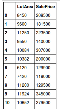

模型

本次使用的是線性回歸模型
y=Wx+by=Wx+b
y=Wx+b
其中WWW為權重，bbb為偏置。
具體地，xxx 即為LotArea，yyy 即為SalePrice。

開始訓練

模型訓練步驟：

1. 設置各種超參數，例如學習率，叠代次數等；
2. 定義變量和模型；
3. 初始化變量;
4. 正式開始訓練.

from __future__ import print_function, division
import tensorflow as tf
import pandas as pd
import numpy as np
import matplotlib.pyplot as plt
import seaborn

# 讀入數據
train = pd.read_csv("Dataset/train.csv")
# 選取房屋面積小於１２０００的數據
train = train[train['LotArea'] < 12000]
train_X = train['LotArea'].values.reshape(-1, 1)
train_Y = train['SalePrice'].values.reshape(-1, 1)

n_samples = train_X.shape[0]
# 學習率
learning_rate = 2
# 叠代次數
training_epochs = 1000
# 每多少次輸出一次叠代結果
display_step = 50

# 這個X和Y和上面的train_X,train_Y是不一樣的，這裏只是個占位符，
# 訓練開始的時候需要“餵”(feed)數據給它
X = tf.placeholder(tf.float32)
Y = tf.placeholder(tf.float32)
# 定義模型參數
W = tf.Variable(np.random.randn(), name="weight", dtype=tf.float32)
b = tf.Variable(np.random.randn(), name="bias", dtype=tf.float32)

# 定義模型
pred = tf.add(tf.mul(W, X), b)
# 定義損失函數
cost = tf.reduce_sum(tf.pow(pred-Y, 2)) / (2 * n_samples)
# 使用Adam算法，至於為什麽不使用一般的梯度下降算法，一會說
optimizer = tf.train.AdamOptimizer(learning_rate).minimize(cost)

# 初始化所有變量
init = tf.initialize_all_variables()

# 訓練開始
with tf.Session() as sess:
    sess.run(init)
    
    for epoch in range(training_epochs):
        for (x, y) in zip(train_X, train_Y):
            sess.run(optimizer, feed_dict={X: x, Y: y})

        if (epoch + 1) % display_step == 0:
            c = sess.run(cost, feed_dict={X: train_X, Y: train_Y})
            print("Epoch:", '%04d' % (epoch + 1), "cost=", "{:.3f}".format(c), "W=", sess.run(W), "b=", sess.run(b))
    
    print("Optimization Finished!")
    training_cost = sess.run(cost, feed_dict={X: train_X, Y: train_Y})
    print("Training cost=", training_cost, "W=", sess.run(W), "b=", sess.run(b), '\n')
    
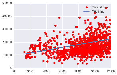
    # 畫圖
    plt.plot(train_X, train_Y, 'ro', label="Original data")
    plt.plot(train_X, sess.run(W) * train_X + sess.run(b), label="Fitted line")
    plt.legend()
    plt.show()

結果如下，

Epoch: 0050 cost= 2283274240.000 W= 20.3469 b= 12945.2
Epoch: 0100 cost= 2196306176.000 W= 19.0349 b= 24402.2
Epoch: 0150 cost= 2128102656.000 W= 17.8766 b= 34479.1
Epoch: 0200 cost= 2074902912.000 W= 16.8604 b= 43292.1
Epoch: 0250 cost= 2033546240.000 W= 15.9735 b= 50965.1
Epoch: 0300 cost= 2001452160.000 W= 15.2026 b= 57622.0
Epoch: 0350 cost= 1976554496.000 W= 14.5348 b= 63380.2
Epoch: 0400 cost= 1957219584.000 W= 13.9577 b= 68350.4
Epoch: 0450 cost= 1942167424.000 W= 13.4598 b= 72634.2
Epoch: 0500 cost= 1930414208.000 W= 13.0309 b= 76322.2
Epoch: 0550 cost= 1921200000.000 W= 12.6619 b= 79494.2
Epoch: 0600 cost= 1913948928.000 W= 12.3445 b= 82220.2
Epoch: 0650 cost= 1908209664.000 W= 12.0717 b= 84562.8
Epoch: 0700 cost= 1903651840.000 W= 11.8377 b= 86572.4
Epoch: 0750 cost= 1900003456.000 W= 11.6364 b= 88299.7
Epoch: 0800 cost= 1897074944.000 W= 11.4638 b= 89781.0
Epoch: 0850 cost= 1894714880.000 W= 11.3161 b= 91048.3
Epoch: 0900 cost= 1892792320.000 W= 11.189 b= 92139.5
Epoch: 0950 cost= 1891217024.000 W= 11.0795 b= 93078.3
Epoch: 1000 cost= 1889932800.000 W= 10.9862 b= 93879.3
Optimization Finished!
Training cost= 1.88993e+09 W= 10.9862 b= 93879.3