ㄧ、資料前處理

1. 補值、刪值

前面我們透過視覺化的方式找到資料有缺值，因此我們要將資料進行補值。要記得訓練資料怎麼補，測試資料也要使用同樣的方法。

補值：在這邊我選擇補-1。一方面是不想和其他資料搞混，補一個大家都沒有的數字。舉例來說有個特徵是工作經驗，你補0就可能與工作經驗0年的搞混。當然補值這種是每個人都有不同想法，所以可以自己去試看看別種方法。

刪值：前面我們有看到有些特徵已經缺值缺了一半以上，那這邊我考慮將他直接刪除，但也可以試試看留下他的特徵將他補值，也許會有不同的效果。

X=df_train.drop(["最高學歷","畢業學校類別","PerStatus"],axis=1)
y=df_train["PerStatus"]
X=X.fillna(-1)
df_test=df_test.fillna(-1)

• 用Smote

  from imblearn.over_sampling import SMOTE
  
  oversample = SMOTE()
  X, y = oversample.fit_resample(X_train, y_train)
  

二、特徵工程

1.將資料做編碼

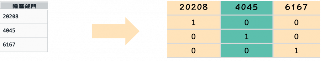
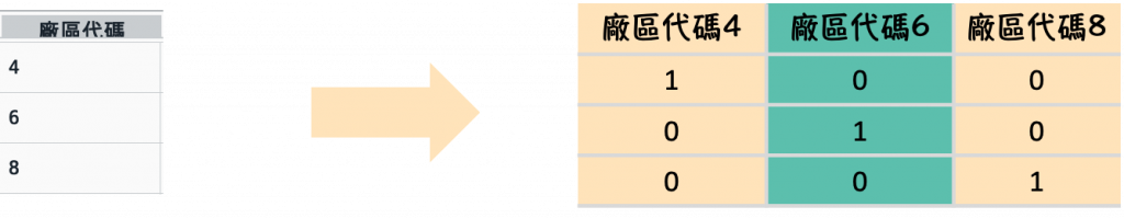
我們分別對廠區代碼以及歸屬部門進行onehot encoding處理

• 歸屬部門（因為歸屬部門眾多，只截出部分結果來示範）

  temp_department=pd.get_dummies(df_X["歸屬部門"],prefix="歸屬部門")
  #%%
  df_X=df_X.drop("歸屬部門",1)
  #%%
  df_X=pd.concat([df_X,temp_department],axis=1)
  

• 廠區代碼（因為廠區代碼眾多，只截出部分結果來示範）

  temp_department=pd.get_dummies(df_X["廠區代碼"],prefix="廠區代碼")
  #%%
  df_X=df_X.drop("廠區代碼",1)
  #%%
  df_X=pd.concat([df_X,temp_department],axis=1)
  

2. 篩選特徵

• 用卡分分配篩選特徵
  我將**?**設為0.01，然後去觀察各個特徵對離職有沒有顯著的影響，然後算出各個特徵值之間的p值，最後有18個特徵符合個特徵符合顯著水準內的0.01

  from sklearn.feature_selection import SelectKBest
  from sklearn.feature_selection import chi2
  best_features = SelectKBest(score_func=chi2, k=10)
  fit = best_features.fit(X, y)
  #%%
  df_scores = pd.DataFrame(fit.scores_)
  df_columns = pd.DataFrame(X.columns)
  #合併
  df_feature_scores = pd.concat([df_columns, df_scores], axis=1)
  #定義列名
  df_feature_scores.columns = ['Feature', 'Score']
  #按照score排序
  df_feature_scores=df_feature_scores.sort_values(by='Score', ascending=False)
  
  #驗證k要用幾個P_value>0.01
  chi_values,pvalues_chi = chi2(X,y)
  K_value = chi_values.shape[0] - (pvalues_chi < 0.01).sum()
  

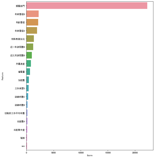
有21個特徵平均分數高於平均

#%%
from sklearn.model_selection import train_test_split
from sklearn.ensemble import RandomForestClassifier
X_train,X_test,y_train,y_test=train_test_split(X,y,test_size=0.3)
rfc=RandomForestClassifier(n_estimators=100,n_jobs = -1,random_state =50, min_samples_leaf = 10)
rfc.fit(X_train, y_train)

df_scores = pd.DataFrame(rfc.feature_importances_)
df_columns = pd.DataFra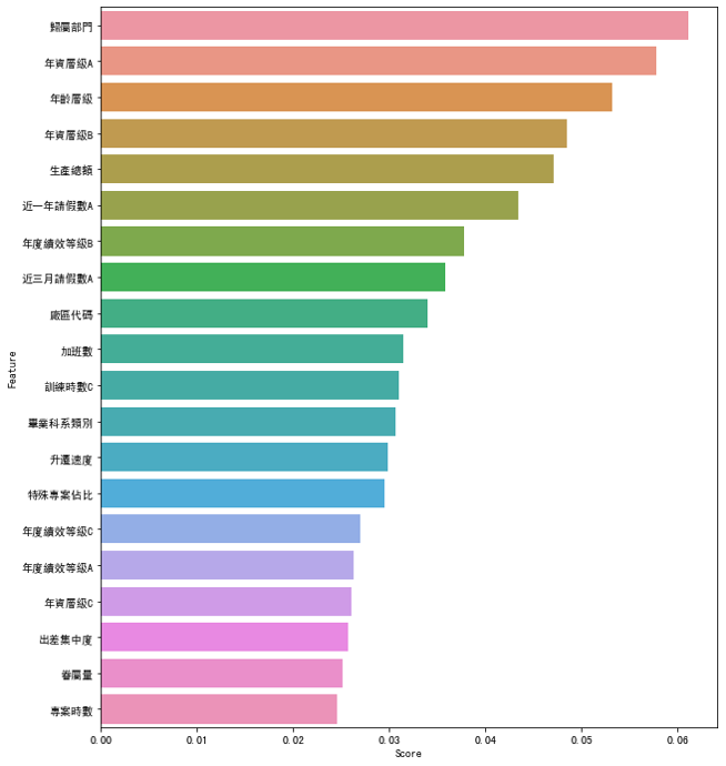![https://ithelp.ithome.com.tw/upload/images/20210908/20140427mHFILo0aDS.png](https://ithelp.ithome.com.tw/upload/images/20210908/20140427mHFILo0aDS.png)me(X.columns)
#合併
df_feature_scores = pd.concat([df_columns, df_scores], axis=1)
#定義列名
df_feature_scores.columns = ['Feature', 'Score']
#按照score排序
df_feature_scores=df_feature_scores.sort_values(by='Score', ascending=False)

#找出有幾個特徵高於平均
num=0
for i in range(0,49):
    if df_scores.iloc[i,0] >= a:
        num=num+1
    else:
        num=num
#畫圖
fig = plt.figure(figsize=(10,12))
#plt.tick_params(axis='x', labelsize=8) 
sns.barplot(df_feature_scores['Score'].head(21),df_feature_scores['Feature'].head(21))

3. 使用PCA進行降維

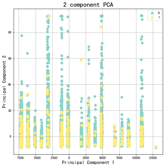
當然我也有將資料轉成2維去試看看，但可以看到PCA無法有效地將離職與非離職之間分開，因此在這筆資料集中這不是一個好的方法。不過就如我們前面所提到的，初期你在做資料分析你一定會試很多方法，到最後你累積經積越多經驗，你就可以看資料來去判斷該用什麼方法。

from sklearn.decomposition import PCA
from sklearn.preprocessing import StandardScaler

X_std = StandardScaler().fit_transform(x)
X_train_std = StandardScaler().fit_transform(X_train)
X_test_std = StandardScaler().fit_transform(X_test)
pca = PCA(0.85)
pca.fit(X_std)
X_train_pca = pca.transform(X_train_std)
X_test_pca = pca.transform(X_test_std)

#%%畫圖
principalDf = pd.DataFrame(data = X_train_pca
             , columns = ['principal component 1', 'principal component 2'])
finalDf = pd.concat([principalDf, up_sample_y], axis = 1)
#%%
cmap = plt.get_cmap('Set3')

#%%
fig = plt.figure(figsize = (8,8))
ax = fig.add_subplot(1,1,1) 
ax.set_xlabel('Principal Component 1', fontsize = 15)
ax.set_ylabel('Principal Component 2', fontsize = 15)
ax.set_title('2 component PCA', fontsize = 20)
targets = [0,1]
colors = cmap(np.linspace(0, 1, len(targets)))
for target, color in zip(targets,colors):
    indicesToKeep = finalDf['PerStatus'] == target
    ax.scatter(finalDf.loc[indicesToKeep, 'principal component 1']
               , finalDf.loc[indicesToKeep, 'principal component 2']
               , c = color
               , s = 50)
ax.legend(targets)
ax.grid()

三、結論

有沒有發現當要把資料丟進模型做訓練前，需要花費大量的時間在整理資料，這也是為什麼我們會在前面花這麼多時間介紹這麼多的處理方法，後面我們將丟入模型去做評估結果囉～