今天我們將稍微講述 Luong 全域注意力機制的原理,並繼續用 Keras 來架構附帶注意力機制的 seq2seq 神經網絡。
Luong attention 機制分為全域( global )和局部( local )兩種策略: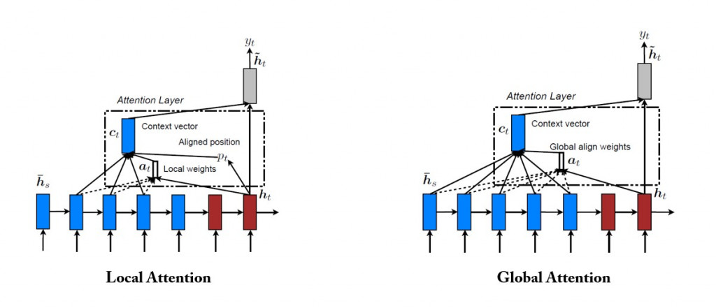
我們採用全域 Luong attention 機制: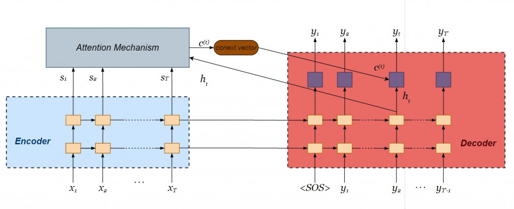
記憶上下文關係的 context vector 為各個單詞的加權平均,其中注意力權重(或稱詞權重)為當下解碼器內部狀態 與各個單詞向量
之間關聯分數出現之機率:
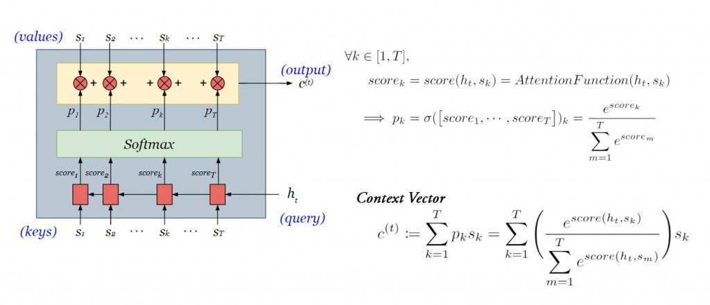
而在前天的文章裡,我們提過三種常見的 attention functions ,今天我們將採用最簡單的點積法。
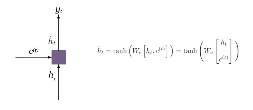
對比附帶注意力機制的編碼器則在遍歷所有的時間點之後僅輸出單一個 context vector ,注意力機制則是針對當下時間點產出 context vector ,每個時間點的 context vector 會不斷更新,有效採計較遙遠的歷史資訊。將解碼器當下的內部狀態和 context vector 連接在一起( concatenate ),經過線性轉換
之後,再經過激活函數
( hyperbolic tangent ),產生專注向量( attentional vector )
,是為 Luong 注意力機制的輸出向量。

圖片來源:https://memes.tw/
你以為事情就這樣結束了嗎?我們還沒得到解碼器最終的輸出值 呢!為了預估當下最有可能出現的單詞,我們還需要透過 softmax 分派機率值到目標語言 word embedding 的各個維度。以下為解碼器的最終步驟:在已知完整來源語言序列
和過往翻譯單詞
的條件下,當下輸出值
出現的條件機率。

理論言畢,接著我們將 Luong (全域)注意力機制加入昨天建構好的雙層 LSTM Encoder-Decoder 網絡。
我們延續Seq2Seq 實作第一篇 的情境,使用以下的英文-西班牙文(雙語)平行語料庫: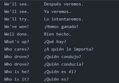
來源語言(英文)的詞向量維度是18(為了方便解說我們使用了 one-hot 編碼,而實務上多用 word2Vec 生成 word embedding ),含有標點符號句長最大值為 4;目標語言(西班牙文)的詞向量則為27,含有句子起始符號 <SOS> 及終止符號 <EOS> 的句長最達值為12。 LSTM 的內部狀態為 256維的向量。我們按照此指定超參數:
### preparing hyperparameters

## source language- English
src_wordEmbed_dim = 18 # dim of text vector representation
src_max_seq_length = 4 # max length of a sentence (including punctuations)

## target language- Spanish
tgt_wordEmbed_dim = 27 # dim of text vector representation
tgt_max_seq_length = 12 # max length of a sentence (including <SOS> and <EOS>)

# dim of context vector
latent_dim = 256
與昨天的編碼器設定大致一樣,唯一不同之處為我們需要將編碼器最上層的輸出值(其實就是各個 LSTM 小單元的 hidden state )傳入注意力層,因而將第二層 LSTM 設定 return_sequences = True 。
### Building a 2-layer LSTM encoder
enc_layer_1 = LSTM(latent_dim, return_sequences = True, return_state = True, name = "1st_layer_enc_LSTM")
# set return_sequence to True so that encoder outputs can be input to attention layer
enc_layer_2 = LSTM(latent_dim, return_sequences = True, return_state = True, name = "2nd_layer_enc_LSTM")
enc_inputs = Input(shape = (src_max_seq_length, src_wordEmbed_dim))
enc_outputs_1, enc_h1, enc_c1 = enc_layer_1(enc_inputs)
enc_outputs_2, enc_h2, enc_c2 = enc_layer_2(enc_outputs_1)
enc_states = [enc_h1, enc_c1, enc_h2, enc_h2]
由於我們將當下的內部狀態 當作 query 傳入注意力層,先刪除原有用來預估當下輸出的激活函數 softmax 。而最上層的 LSTM 也不必回傳內部狀態,因此設定 return_state = False 。
### Building a 2-layer LSTM decoder
dec_layer_1 = LSTM(latent_dim, return_sequences = True, return_state = True, name = "1st_layer_dec_LSTM")
dec_layer_2 = LSTM(latent_dim, return_sequences = True, return_state = False, name = "2nd_layer_dec_LSTM")
dec_dense = Dense(tgt_wordEmbed_dim, activation = "softmax")
dec_inputs = Input(shape = (tgt_max_seq_length, tgt_wordEmbed_dim))
dec_outputs_1, dec_h1, dec_c1 = dec_layer_1(dec_inputs, initial_state = [enc_h1, enc_c1])
dec_outputs_2 = dec_layer_2(dec_outputs_1, initial_state = [enc_h2, enc_c2])
from tensorflow.keras.layers import dot

attention_scores = dot([dec_outputs_2, enc_outputs_2], axes = [2, 2])
from tensorflow.keras.layers import Activation

attenton_weights = Activation("softmax")(attention_scores)
print("attention weights - shape: {}".format(attenton_weights.shape)) # shape: (None, enc_max_seq_length, dec_max_seq_length)
context_vec = dot([attenton_weights, enc_outputs_2], axes = [2, 1])
print("context vector - shape: {}".format(context_vec.shape)) # shape: (None, dec_max_seq_length, latent_dim)
# concatenate context vector and decoder hidden state h_t
ht_context_vec = concatenate([context_vec, dec_outputs_2], name = "concatentated_vector")
print("ht_context_vec - shape: {}".format(ht_context_vec.shape)) # shape: (None, dec_max_seq_length, 2 * latent_dim)

# obtain attentional vector
attention_vec = Dense(latent_dim, use_bias = False, activation = "tanh", name = "attentional_vector")(ht_context_vec)
print("attention_vec - shape: {}".format(attention_vec.shape)) # shape: (None, dec_max_seq_length, latent_dim)
將注意力機制的輸出值傳入 softmax 層得到當下的目標詞向量:
dec_outputs_final = Dense(tgt_wordEmbed_dim, use_bias = False, activation = "softmax")(attention_vec)
print("dec_outputs_final - shape: {}".format(dec_outputs_final.shape)) # shape: (None, dec_max_seq_length, tgt_wordEmbed_dim)
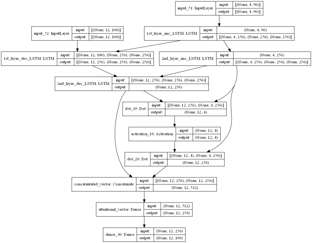
我們使用 tf.keras.models.Model 物件,指定模型的輸入(與未附加注意力機制的 seq2seq 相通)與模型的輸出,將 encoder 、 decoder 以及 attention layer 三者串連起來,並使用 plot_model 函式畫出模型的架構:
from tensorflow.keras.utils import plot_model

# Integrate seq2seq model with attention mechanism
seq2seq_2_layers_attention = Model([enc_inputs, dec_inputs], dec_outputs_final, name = "seq2seq_2_layers_attention")
seq2seq_2_layers.summary()

# Preview model architecture
plot_model(seq2seq_2_layers_attention, to_file = "output/2-layer_seq2seq_attention.png", dpi = 100, show_shapes = True, show_layer_names = True)
以上我們示範了如何利用 Keras API 建構出附帶 Luong 全域注意力機制的 LSTM seq2seq 的神經網絡。由於時間有限,我們得先停在這裡,而仍有以下殘留課題:
各位有個美好的周末嗎?我們明天見!


 iThome鐵人賽