今天的內容依舊為訓練翻譯 seq2seq 神經網絡的歷程( training process )。
機器學習的兩大階段-訓練(training)與推論(inference):
圖片來源:www.intel.com
為了避免在稍後建立 numpy array 時耗掉所有的 RAM ( out of memory, OOM ),我們將資料量縮減為10000筆(資料瘦身之後 max_seq_length 、vocab_size 也會跟著改變):
# reduce size of seq_pairs
n_samples = 10000
seq_pairs = seq_pairs[:n_samples]


"""
Evaluating max_seq_length and vocab_size for both English and Chinese ...
Results are given as follows:
    src_max_seq_length = 13
    tgt_max_seq_length = 22
    src_vocab_size == 3260   # 3260 unique tokens in total
    tgt_vocab_size == 2504   # 2504 unique tokens in total
"""
我們之後會將經過斷詞之後的句子當作輸入傳入 seq2seq 模型並經過 word embedding 轉為低維度的向量,因此不論是針對編碼器或是解碼器的輸入句子(原型態為 string )我們都會進行 label encoding (將每個斷開的單詞賦予詞彙表中的編號)。 由於翻譯模型將每個經過 label encoding 的單詞對應到目標詞彙表中的某個單詞,因此翻譯任務本身可視為一個多類別的分類問題,而類別數量即是目標語言的單詞總數( tgt_vocab_size )。我們很自然地將解碼器的輸出單詞進行 one-hot 編碼。
def encode_input_sequences(tokeniser, max_seq_length, sentences):
    """
    Label encode every sentences to create features X
    """
    # label encode every sentences
    sentences_le = tokeniser.texts_to_sequences(sentences)
    # pad sequences with zeros at the end
    X = pad_sequences(sentences_le, maxlen = max_seq_length, padding = "post")
    return X


def encode_output_labels(sequences, vocab_size):
    """
    One-hot encode target sequences to create labels y
    """
    y_list = []
    for seq in sequences:
        # one-hot encode each sentence
        oh_encoded = to_categorical(seq, num_classes = vocab_size)
        y_list.append(oh_encoded)
    y = np.array(y_list, dtype = np.float32)
    y = y.reshape(sequences.shape[0], sequences.shape[1], vocab_size)
    return y

# create encoder inputs, decoder inputs and decoder outputs
enc_inputs = encode_input_sequences(src_tokeniser, src_max_seq_length, src_sentences) # shape: (n_samples, src_max_seq_length, 1)
dec_inputs = encode_input_sequences(tgt_tokeniser, tgt_max_seq_length, tgt_sentences) # shape: (n_samples, tgt_max_seq_length, 1)
dec_outputs = encode_input_sequences(tgt_tokeniser, tgt_max_seq_length, tgt_sentences)
dec_outputs = encode_output_labels(dec_outputs, tgt_vocab_size) # shape: (n_samples, tgt_max_seq_length, tgt_vocab_size )
Label Encoding為類別編號,產生一個純量;One-Hot Encoding 則是對應該類別的維度為1,其餘維度皆為0,產生一個n維向量(n為類別總數):
圖片來源:medium.com
將建立好的特徵 enc_inputs 、 dec_inputs 以及標籤 dec_outputs 連同來源語言(英文)的詞彙總數 src_vocab_size 以上資訊一並存入同一份壓縮 .npz 格式以便後續訓練模型時可快速取用,並以其在現有程式中的變數名稱當作引數名稱(用以查找個別檔案之關鍵字):
# save required data to a compressed file
np.savez_compressed("data/eng-cn_data.npz", enc_inputs = enc_inputs, dec_inputs = dec_inputs, dec_outputs = dec_outputs, src_vocab_size = src_vocab_size)
載入之前寫入壓縮檔的合併訓練資料,必且按照檔案關鍵字還原個別的 Numpy arrays :
import numpy as np

data = np.load("data/eng-cn_data.npz")
print(data.files) # ['enc_inputs', 'dec_inputs', 'dec_outputs', 'src_vocab_size']

# Extract our desired data
enc_inputs = data["enc_inputs"]
dec_inputs = data["dec_inputs"]
dec_outputs = data["dec_outputs"]
src_vocab_size = data["src_vocab_size"].item(0)
注意此時的 enc_inputs 、 dec_inputs 和 dec_outputs 依舊是按照原始語料庫中的前10000筆進行排列,我們建立 shuffler 並用它來打亂排列順序,同時保留資料中每個句子的對應關係:
# shuffle X and y in unision
shuffler = np.random.permutation(enc_inputs.shape[0])
enc_inputs = enc_inputs[shuffler]
dec_inputs = dec_inputs[shuffler]
dec_outputs = dec_outputs[shuffler]
我們可以使用 sklearn.model_selection 模組當中定義的 train_test_split() 函式將資料依照指定的比例分割成訓練資料以及測試資料,在此我們將原有資料的 20% 劃為測試用資料:
from sklearn.model_selection import train_test_split


# prepare training and test data
test_ratio = .2
enc_inputs_train, enc_inputs_test = train_test_split(enc_inputs, test_size = test_ratio, shuffle = False)
dec_inputs_train, dec_inputs_test = train_test_split(dec_inputs, test_size = test_ratio, shuffle = False)
y_train, y_test = train_test_split(dec_outputs, test_size = test_ratio, shuffle = False)
X_train = [enc_inputs_train, dec_inputs_train]
X_test = [enc_inputs_test, dec_inputs_test]
準備好訓練以及測試用的特徵以及標籤之後,我們就可以來建立模型了。
從 enc_inputs 與 dec_outputs 的維度資訊可以得到中英文的最大序列長度(可理解為最大的句子長度)以及目標單詞的詞彙總數(這也是為什麼我們需要特別再存入 src_vocab_size ):
src_max_seq_length = enc_inputs.shape[1]
tgt_max_seq_length = dec_outputs.shape[1]
tgt_vocab_size = dec_outputs.shape[2]
指定英文和中文的 embedding 維度以及 LSTM 內部狀態向量的維度等超參數,我們可由以上超參數以及中、英文最大序列長度和英文詞彙總數 src_vocab_size 來建立一個附帶 Luong attention 機制雙層 LSTM seq2seq 神經網絡。自定函式build_seq2seq()將建立神經網絡之外,緊接著指定衡量預測值與實際值之間誤差的損失函數(由於輸出值 dec_outputs 為 one-hot 編碼向量,我們指定損失函數為適用於多類別分類問題的 CategoricalCrossentropy()) 並定義找尋損失函數最小值使用的梯度下降演算法為 Adam ,指定其學習率( learning rate,其也是可 fine-tune 的超參數之一)。
# hyperparameters
src_wordEmbed_dim = 96
tgt_wordEmbed_dim = 100
latent_dim = 256

def build_seq2seq(src_max_seq_length, src_vocab_size, src_wordEmbed_dim, tgt_max_seq_length, tgt_vocab_size, tgt_wordEmbed_dim, latent_dim, model_name = None):
    """
    Builda an LSTM seq2seq model with Luong attention
    """
    # Build an encoder
    enc_inputs = Input(shape = (src_max_seq_length, ))
    vectors = Embedding(input_dim = src_vocab_size, output_dim = src_wordEmbed_dim, name = "embedding_enc")(enc_inputs)
    enc_outputs_1, enc_h1, enc_c1 = LSTM(latent_dim, return_sequences = True, return_state = True, name = "1st_layer_enc_LSTM")(vectors)
    enc_outputs_2, enc_h2, enc_c2 = LSTM(latent_dim, return_sequences = True, return_state = True, name = "2nd_layer_enc_LSTM")(enc_outputs_1)
    enc_states = [enc_h1, enc_c1, enc_h2, enc_h2]

    # Build a decoder
    dec_inputs = Input(shape = (tgt_max_seq_length, ))
    vectors = Embedding(input_dim = tgt_vocab_size, output_dim = tgt_wordEmbed_dim, name = "embedding_dec")(dec_inputs)
    dec_outputs_1, dec_h1, dec_c1 = LSTM(latent_dim, return_sequences = True, return_state = True, name = "1st_layer_dec_LSTM")(vectors, initial_state = [enc_h1, enc_c1])
    dec_outputs_2 = LSTM(latent_dim, return_sequences = True, return_state = False, name = "2nd_layer_dec_LSTM")(dec_outputs_1, initial_state = [enc_h2, enc_c2])

    # evaluate attention score
    attention_scores = dot([dec_outputs_2, enc_outputs_2], axes = [2, 2])
    attenton_weights = Activation("softmax")(attention_scores)
    context_vec = dot([attenton_weights, enc_outputs_2], axes = [2, 1])
    ht_context_vec = concatenate([context_vec, dec_outputs_2], name = "concatentated_vector")
    attention_vec = Dense(latent_dim, use_bias = False, activation = "tanh", name = "attentional_vector")(ht_context_vec)
    logits = TimeDistributed(Dense(tgt_vocab_size))(attention_vec)
    dec_outputs_final = Activation("softmax", name = "softmax")(logits)

    # integrate as a model
    model = Model([enc_inputs, dec_inputs], dec_outputs_final, name = model_name)
    # compile model
    model.compile(
        optimizer = tf.keras.optimizers.Adam(learning_rate = 1e-3),
        loss = tf.keras.losses.CategoricalCrossentropy(),
    )
    return model

# build our seq2seq model
eng_cn_translator = build_seq2seq(
    src_max_seq_length = src_max_seq_length,
    src_vocab_size = src_vocab_size,
    src_wordEmbed_dim = src_wordEmbed_dim,
    tgt_max_seq_length = tgt_max_seq_length,
    tgt_vocab_size = tgt_vocab_size,
    tgt_wordEmbed_dim = tgt_wordEmbed_dim,
    latent_dim = latent_dim,
    model_name = "eng-cn_translator_v1"
    )
eng_cn_translator.summary()
模型中可經過反向傳播( backpropagation, BP )進行學習的參數有3,115,624個,構成了決定此模型的所有參數: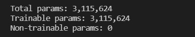
檢查模型架構中各層神經元輸入與輸出的維度是否正確: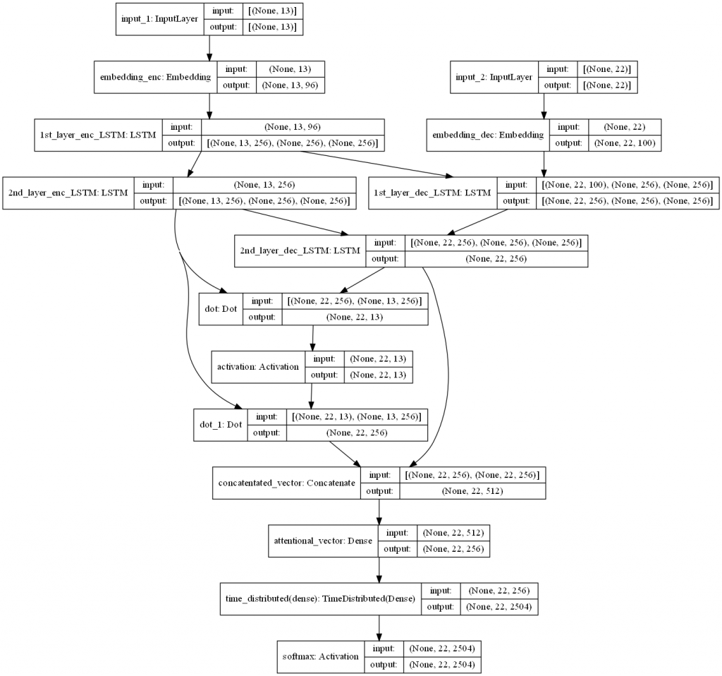
我們希望記錄訓練過程中的模型權重( model weights )變化以及模型本身(以 .h5 格式呈現),加入了 tf.keras.callbacks.ModelCheckpoint 物件。如此之外,我們也希望在訓練過程中若是誤差(損失函數)超過10個訓練期依舊持續停止下降即中止模型訓練,引入 tf.keras.callbacks.EarlyStopping 物件。我們將讓模型學習訓練資料X_train = [enc_inputs_train, dec_inputs_train]和y_train,並且取其中的 20% 當作驗證資料:
# save model and its weights at a certain frequency
ckpt = ModelCheckpoint(
    filepath = "models/eng-cn_translator_v1.h5",
    monitor = "val_loss",
    verbose = 1,
    save_best_only = True,
    save_weights_only = False,
    save_freq = "epoch",
    mode = "min",
)
es = EarlyStopping(
    monitor = "loss",
    mode = "min",
    patience = 10
)

# train model
train_hist = eng_cn_translator.fit(
                            X_train,
                            y_train,
                            batch_size = 64,
                            epochs = 200,
                            validation_split = .2,
                            verbose = 2,
                            callbacks = [es, ckpt]
                        )

# preview training history
print("training history have info: {}".format(train_hist.history.keys())) # ['loss', 'val_loss']
fig, ax = plt.subplots(figsize = (10, 5))
fig.suptitle("Eng-Cn NMT Model")
ax.set_title("Cross Entropy Loss")
ax.plot(train_hist.history["loss"], label = "train")
ax.plot(train_hist.history["val_loss"], label = "validation")
ax.set_xlabel("epoch")
ax.set_ylabel("func value")
ax.legend()
plt.show()
經過了200個 epochs (一個 epoch 為一次 feed forward 得到輸出加上一次 back propagation 更新參數),我們可以觀察模型在訓練資料集上與驗證資料集上誤差的遞減: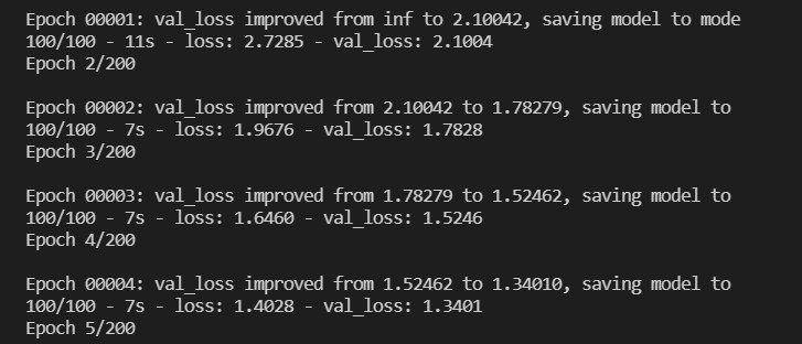
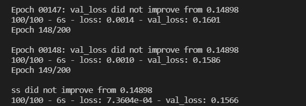
訓練好之後即回顧訓練中每個時期( epoch )中損失函數下降變化: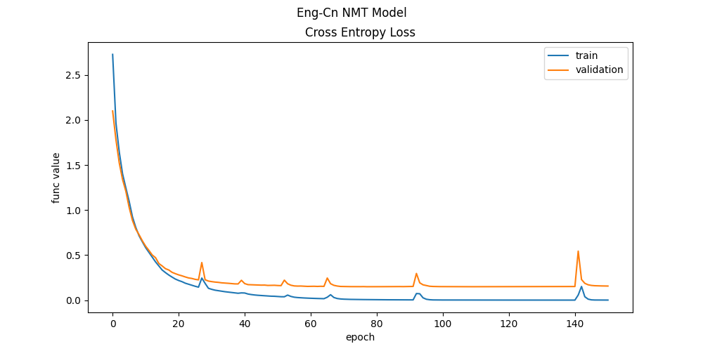
模型訓練好了,下一步就是評估模型好壞的時刻。我們將透過計算模型在語料庫中的 BLEU (bilingual evaluation understudy) 得分來衡量此 seq2seq 模型的翻譯品質。今天的實作進度就到此告一段落,bis morgen und gute Nacht!