前言

我們緊接著切入 RNN 為架構的編碼器-解碼器。

在seq2seq之前

RNN Encoder-Decoder

在 Google 正式提出 seq2seq 架構之前， Cho 等人就提出了以標準循環神經網絡（ standard RNN ）設計編碼器-解碼器的演算法：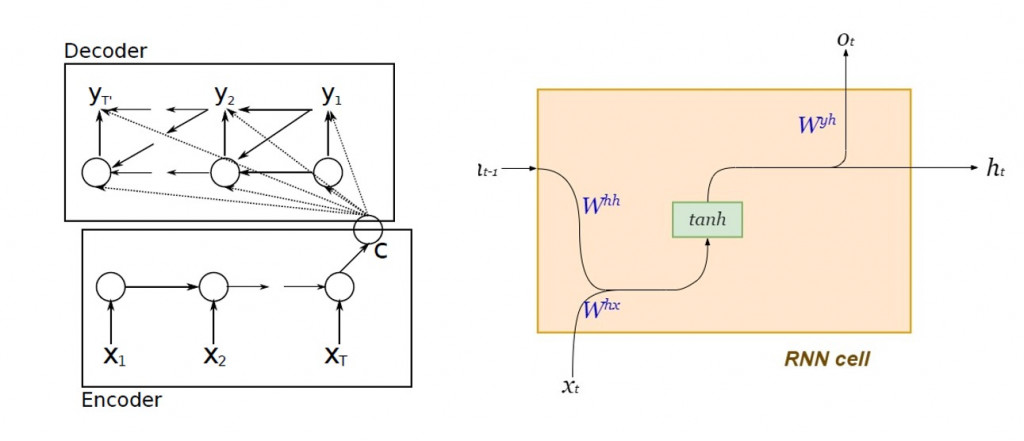

圖片來源：Learning Phrase Representations using RNN Encoder–Decoder for Statistical Machine Translation

編碼器及解碼器內部的動態系統方程：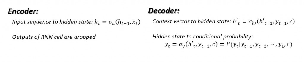

其用意是為了以最大似然（ maximum likelihood ）估計來條件機率：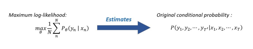

單層LSTM Encoder-Decoder

最簡單的 seq2seq 編碼器內部由一層 LSTM 細胞串聯而成，下圖右方為每個 LSTM 細胞內部的結構以及其動態方程：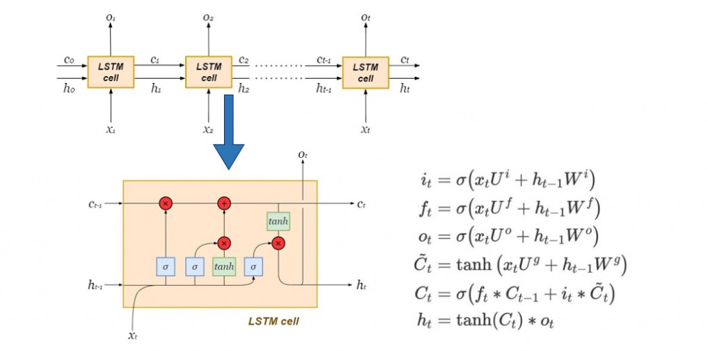

雖然傳統 RNN 的內部隱藏狀態（ hidden state ）能夠保存上下文關係，然而在輸入的單詞序列過長時，距離預測愈遙遠的歷史訊息幾乎已無發揮影響力，將會發生梯度消失（ vanishing gradient ），在長句的翻譯上未能達到令人滿意的效果。而 LSTM 保留了 RNN 原有的隱藏狀態，並加入了細胞狀態（ cell state ）來記錄距離預測值遙遠的歷史資訊，以實現長期依賴（ long-term dependency ）。

Hidden state捕捉短期記憶，而cell state則儲存長期記憶：
Characterization is an abstract term that merely serves to illustrate how the hidden state is more concerned with the most recent time-step. The cell state is basically the global or aggregate memory of the LSTM network over all time-steps.

文字出處：LSTMs Explained: A Complete, Technically Accurate, Conceptual Guide with Keras

寫一個簡單的seq2seq網絡吧

接下來我們將使用 Tensorflow 建立單層的 LSTM seq2seq 。在這裡我們先示範如何利用 Keras API 的模型定義編碼器及解碼器，而不細談文本的來源與文字前處理，以及如何直接使用 Tensorflow 基本語法建立 seq2seq 模型。

我們以翻譯作為前提，考慮意義相同的來源語言文句以及目標語言文句並行條列而成的雙語平行文本（如下圖所示）：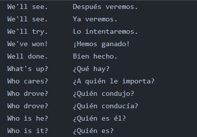

資料準備

首先要確立的是編碼器輸入資料的張量維度「 來源語言文句總數 × 來源語言中最長文句之詞條數量 × 來源語言內撇除重複詞條的總數 」，並指定資料型態為單精確浮點數 float32：

import numpy as np
from preprocess_text import input_docs, target_docs, input_tokens, target_tokens, num_encoder_tokens, num_decoder_tokens, max_encoder_seq_length, max_decoder_seq_length

encoder_input_data = np.zeros(
    shape = (len(input_docs), max_encoder_seq_length, num_encoder_tokens),
    dtype = "float32"
    )

接下來確立解碼器輸入資料的張量維度「 來源語言文句總數 × 目標語言最長文句之詞條數量 × 目標語言內撇除重複詞條的總數 」以及輸出資料的張量維度「 目標語言文句總數 × 目標語言最長文句之詞條數量 × 目標語言內撇除重複詞條的總數 」

# Build out the decoder_input_data matrix:
decoder_input_data = np.zeros(
    (len(input_docs), max_decoder_seq_length, num_decoder_tokens),
    dtype = "float32"
    )
# Build out the decoder_target_data matrix:
decoder_target_data = np.zeros(
    (len(target_docs), max_decoder_seq_length, num_decoder_tokens),
    dtype = "float32"
    )

接下來將單詞表示為向量，並依照前後順序（建立時間序列），填入剛才建立的 NumPy 陣列！雖然在實務應用上，翻譯任務的詞彙表通常極為龐大，往往使用word2Vec 進行 word embedding 到相對低維度的向量，但在這裡我們採用 one-hot 編碼，因此單詞向量之維度便是文本詞彙量。

# since we're using a bilingual parallel corpus, we have the same number of sentences in both languages, therefore same size of input and target documents
for line, (input_doc, target_doc) in enumerate(zip(input_docs, target_docs)):
    for timestep, token in enumerate(re.findall(r"[\w']+|[^\s\w]", input_doc)):
        encoder_input_data[line, timestep, input_features_dict[token]] = 1.
    for timestep, token in enumerate(target_doc.split()):
        decoder_input_data[line, timestep, target_features_dict[token]] = 1.
        if timestep > 0:
            decoder_target_data[line, timestep - 1, target_features_dict[token]] = 1.

今天的介紹就先寫到這裡，明天繼續！

閱讀更多

1. Learning Phrase Representations using RNN Encoder-Decoder for Statistical Machine Translation
2. Keras API- LSTM