別想太多,做就對了!
《捍衛戰士:獨行俠》
前兩天我們已經了解 BERT 的內部運作,還有 BERT 在進行語言處理上的一些缺陷。今天不聊理論,我們來簡單一一解析 Tensorflow 的官方教學 沒錯,又是 Tensorflow 了喔,並結合前兩天所學到的知識,來對教學中程式碼進行剖析。由於 BERT 的應用實在太多了,所以今天只會提到最簡單的情緒文本分析,也就是先前所說的多對一文本分類,若各位有興趣,或許我們明年還可以相見?在下面留言:)
今天的程式碼將會全部取自於 Tensorflow 官方教學文件。
在開始進入正題之前,我們得先在 Colab 中建置環境。Colab 是線上的編譯工具,也是機器學習常用的程式平台,更是初學者剛學習 Python 的最佳途徑。之所以 ML 常用,是因為在上面可以調用 Google 分配的運算資源,讓運算速度可以比較快一點。在開始之前,讓我們先來建置一下環境。
# A dependency of the preprocessing for BERT inputs
pip install -q -U "tensorflow-text==2.8.*"
pip install -q tf-models-official==2.7.0
搭建 BERT 通常會需要兩個步驟:資料前處理、模型建置。在這裡的資料前處理跟先前我們所學利用正規表達式來清理資料的那種前處理有一點差別。還記得我們先前學習正規表達式的時候,是為了要將文本中不需要的詞以及符號等等的刪除,只留下我們所需要的資料即可;但在搭建 BERT 時,所謂的前處理就不再是指清理資料了,而是將資料轉換成 BERT 可以理解的格式。
接著我們在這邊將需要的套件引入程式中。
import os
import shutil
# 這兩個套件是為了要將訓練資料的路徑讀取工具也引進來

import tensorflow as tf # 就是 Tensorflow 不用多說
import tensorflow_hub as hub # Tensorflow bert 社群
import tensorflow_text as text # 前處理
from official.nlp import optimization  # 優化工具

import matplotlib.pyplot as plt # 畫圖用的套件

tf.get_logger().setLevel('ERROR') # Debug的工具,也可以不寫
接下來就是要引入訓練的資料。我們在這邊引用網路上常用的 imdb 情感分析資料。在這邊可以看到套件 os 是為了要將路徑整合,使模型可以更方便讀取我們下載的訓練資料。
# 這個是資料集的下載連結,如果你複製這段 url 到瀏覽器上,也可以下載的到
url = 'https://ai.stanford.edu/~amaas/data/sentiment/aclImdb_v1.tar.gz'

dataset = tf.keras.utils.get_file('aclImdb_v1.tar.gz', url,
                                  untar=True, cache_dir='.',
                                  cache_subdir='')

# 所謂的 os.path.join 就是把兩個路徑結合起來的意思,如果路徑是 ./data/,join之後就會變成 ./data/aclImdb,而以下所做的,就是要整合資料路徑,方便之後模型讀取
dataset_dir = os.path.join(os.path.dirname(dataset), 'aclImdb')

train_dir = os.path.join(dataset_dir, 'train')

# remove unused folders to make it easier to load the data
remove_dir = os.path.join(train_dir, 'unsup')
shutil.rmtree(remove_dir)
Downloading data from https://ai.stanford.edu/~amaas/data/sentiment/aclImdb_v1.tar.gz
84131840/84125825 [==============================] - 7s 0us/step
84140032/84125825 [==============================] - 7s 0us/step
接下來就是把資料轉換成訓練資料集以及測試資料集,在這裡我們將資料以 8:2 的形式,將資料進行分割。官方文件是透過 keras 的 text_dataset_from_directory 函式中的一個參數來分割資料。至於所謂的 batch_size 就是每一批放進模型訓練的批量。
AUTOTUNE = tf.data.AUTOTUNE
batch_size = 32
seed = 42

raw_train_ds = tf.keras.utils.text_dataset_from_directory(
    'aclImdb/train',
    batch_size=batch_size,
    validation_split=0.2,
    subset='training',
    seed=seed)

class_names = raw_train_ds.class_names
train_ds = raw_train_ds.cache().prefetch(buffer_size=AUTOTUNE)

val_ds = tf.keras.utils.text_dataset_from_directory(
    'aclImdb/train',
    batch_size=batch_size,
    validation_split=0.2,
    subset='validation',
    seed=seed)

val_ds = val_ds.cache().prefetch(buffer_size=AUTOTUNE)

test_ds = tf.keras.utils.text_dataset_from_directory(
    'aclImdb/test',
    batch_size=batch_size)

test_ds = test_ds.cache().prefetch(buffer_size=AUTOTUNE)
Found 25000 files belonging to 2 classes.
Using 20000 files for training.
Found 25000 files belonging to 2 classes.
Using 5000 files for validation.
Found 25000 files belonging to 2 classes.
最後我們可以得到訓練資料集 train_ds 以及驗證資料集 val_ds,以及最後的測試資料集 test_ds。如果我們看一下裡面的資料長什麼樣子,就會發現0代表負面影評,1代表正面影評。
for text_batch, label_batch in train_ds.take(1):
   print(f'Review: {text_batch.numpy()[0]}')
   label = label_batch.numpy()[i]
   print(f'Label : {label} ({class_names[label]})')
這邊就不印出三份資料了,印出第一份讓大家來有點概念即可。
Review: b'"Pandemonium" is a horror movie spoof that comes off more stupid than funny. Believe me when I tell you, I love comedies. Especially comedy spoofs. "Airplane", "The Naked Gun" trilogy, "Blazing Saddles", "High Anxiety", and "Spaceballs" are some of my favorite comedies that spoof a particular genre. "Pandemonium" is not up there with those films. Most of the scenes in this movie had me sitting there in stunned silence because the movie wasn\'t all that funny. There are a few laughs in the film, but when you watch a comedy, you expect to laugh a lot more than a few times and that\'s all this film has going for it. Geez, "Scream" had more laughs than this film and that was more of a horror film. How bizarre is that?<br /><br />*1/2 (out of four)'
Label : 0 (neg)
記得我們先前所說的遷移學習(Transfer Learning)嗎?我們可以取用別人已經訓練好的預訓練模型,再針對預訓練模型加上我們自己的資料,讓模型找出特徵之後,來解決自然語言處理的下游任務。那該要到哪裡去下載別人已經預訓練好的模型呢?網路上有兩個常用的平台,一個是我們現在用的 Tensorflow 的 hub ,另一個則是大家更常用的抱臉怪(huggingface),在抱臉怪上有各式各樣別人從各領域的文本所訓練的預訓練模型,而大家可以在上面任意取用符合自己需求的預訓練模型。
而以下所做的,就是取用別人已經訓練好的模型,並把它用在我們的任務當中。
tfhub_handle_encoder = "https://tfhub.dev/tensorflow/small_bert/bert_en_uncased_L-4_H-512_A-8/1" # 這是預訓練模型
tfhub_handle_preprocess = "https://tfhub.dev/tensorflow/bert_en_uncased_preprocess/3" # 這是 BERT 前處理需要用的模型
以下就可以來研究看看輸入進去的資料會有哪些。
bert_preprocess_model = hub.KerasLayer(tfhub_handle_preprocess) # 呼叫前處理模型
text_test = ['this is such an amazing movie!'] # 先輸入簡單的句子看看會變成什麼樣子
text_preprocessed = bert_preprocess_model(text_test)
print(f'Keys       : {list(text_preprocessed.keys())}')
print(f'Shape      : {text_preprocessed["input_word_ids"].shape}')
print(f'Word Ids   : {text_preprocessed["input_word_ids"][0, :12]}')
print(f'Input Mask : {text_preprocessed["input_mask"][0, :12]}')
print(f'Type Ids   : {text_preprocessed["input_type_ids"][0, :12]}')
Keys       : ['input_type_ids', 'input_word_ids', 'input_mask']
Shape      : (1, 128)
Word Ids   : [ 101 2023 2003 2107 2019 6429 3185  999  102    0    0    0]
Input Mask : [1 1 1 1 1 1 1 1 1 0 0 0]
Type Ids   : [0 0 0 0 0 0 0 0 0 0 0 0]
我們可以看到輸出總共分成 input_word_ids、input_mask、以及 input_type_ids。其中input_word_ids就是每個文字分配的識別碼,可以讓模型分別對應回去的數字。 input_mask 則是在進行 Masked 的程序(我的理解,若有錯還請不吝賜教),而input_type_ids則是會依照不同句子給予不同的id,也就是識別句子的功能。這邊是因為測試的句子只有一句,所以只會有 0 這個數字。
bert_model = hub.KerasLayer(tfhub_handle_encoder)
bert_results = bert_model(text_preprocessed)
print(f'Loaded BERT: {tfhub_handle_encoder}')
print(f'Pooled Outputs Shape:{bert_results["pooled_output"].shape}')
print(f'Pooled Outputs Values:{bert_results["pooled_output"][0, :12]}')
print(f'Sequence Outputs Shape:{bert_results["sequence_output"].shape}')
print(f'Sequence Outputs Values:{bert_results["sequence_output"][0, :12]}')
Loaded BERT: https://tfhub.dev/tensorflow/small_bert/bert_en_uncased_L-4_H-512_A-8/1
Pooled Outputs Shape:(1, 512)
Pooled Outputs Values:[ 0.76262873  0.99280983 -0.1861186   0.36673835  0.15233682  0.65504444
  0.9681154  -0.9486272   0.00216158 -0.9877732   0.0684272  -0.9763061 ]
Sequence Outputs Shape:(1, 128, 512)
Sequence Outputs Values:[[-0.28946388  0.3432126   0.33231565 ...  0.21300787  0.7102078
  -0.05771166]
 [-0.28742015  0.31981024 -0.2301858  ...  0.58455074 -0.21329722
   0.7269209 ]
 [-0.66157013  0.6887685  -0.87432927 ...  0.10877253 -0.26173282
   0.47855264]
 ...
 [-0.2256118  -0.28925604 -0.07064401 ...  0.4756601   0.8327715
   0.40025353]
 [-0.29824278 -0.27473143 -0.05450511 ...  0.48849759  1.0955356
   0.18163344]
 [-0.44378197  0.00930723  0.07223766 ...  0.1729009   1.1833246
   0.07897988]]
在輸出中,總共有三個不同需要注意的欄位:pooled_output、sequence_output、encoder_outputs。
pooled_output:代表所有資料經由 BERT 之後所取出的 embedding。在這裡代表的就是電影評論資料整體的 embedding。sequence_output:代表的是每一個 token 在上下文中的 embedding。透過 BERT 取得了需要的 embedding 之後,接下來就是要進行下游任務,在這裡就是進行文本分類。
Tutorial 在這裡用一個函式來定義模型搭建:
def build_classifier_model():
  text_input = tf.keras.layers.Input(shape=(), dtype=tf.string, name='text')
  preprocessing_layer = hub.KerasLayer(tfhub_handle_preprocess, name='preprocessing')
  encoder_inputs = preprocessing_layer(text_input)
  encoder = hub.KerasLayer(tfhub_handle_encoder, trainable=True, name='BERT_encoder')
  outputs = encoder(encoder_inputs)
  net = outputs['pooled_output']
  net = tf.keras.layers.Dropout(0.1)(net)
  net = tf.keras.layers.Dense(1, activation=None, name='classifier')(net)
  return tf.keras.Model(text_input, net)
模型架構如下: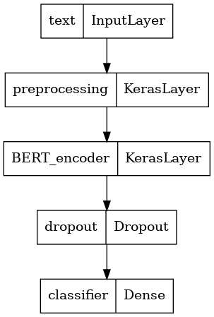
Source: Tensorflow
接下來就是要用 Cross entropy 來計算損失函數,前面沒有介紹到損失函數。簡單的說,損失函數就是在進行梯度下降時,模型在評估與正確答案的相近程度時所計算的最小化最佳解問題,即為負對數似然(negative log-likelihood)。
接著設定後面的模型參數。Learning rate 則採取原論文建議的參數:3e-5。原論文建議三種參數,分別為5e-5、3e-5、2e-5。至於 epoch、batch、以及 learning rate,大家可以來看這位前輩寫的文章。最後在這裡將優化參數加進 create_optimizer 函式中,以利後續在編譯時對模型進行優化。
loss = tf.keras.losses.BinaryCrossentropy(from_logits=True)
metrics = tf.metrics.BinaryAccuracy()

epochs = 5
steps_per_epoch = tf.data.experimental.cardinality(train_ds).numpy()
num_train_steps = steps_per_epoch * epochs
num_warmup_steps = int(0.1*num_train_steps)

init_lr = 3e-5
optimizer = optimization.create_optimizer(init_lr=init_lr,
                                          num_train_steps=num_train_steps,
                                          num_warmup_steps=num_warmup_steps,
                                          optimizer_type='adamw')
最後就是開始訓練:
classifier_model.compile(optimizer=optimizer,
                         loss=loss,
                         metrics=metrics)
print(f'Training model with {tfhub_handle_encoder}')
history = classifier_model.fit(x=train_ds,
                               validation_data=val_ds,
                               epochs=epochs)
Training model with https://tfhub.dev/tensorflow/small_bert/bert_en_uncased_L-4_H-512_A-8/1
Epoch 1/5
625/625 [==============================] - 90s 136ms/step - loss: 0.4784 - binary_accuracy: 0.7528 - val_loss: 0.3713 - val_binary_accuracy: 0.8350
Epoch 2/5
625/625 [==============================] - 83s 133ms/step - loss: 0.3295 - binary_accuracy: 0.8525 - val_loss: 0.3675 - val_binary_accuracy: 0.8472
Epoch 3/5
625/625 [==============================] - 83s 133ms/step - loss: 0.2503 - binary_accuracy: 0.8963 - val_loss: 0.3905 - val_binary_accuracy: 0.8470
Epoch 4/5
625/625 [==============================] - 83s 133ms/step - loss: 0.1930 - binary_accuracy: 0.9240 - val_loss: 0.4566 - val_binary_accuracy: 0.8506
Epoch 5/5
625/625 [==============================] - 83s 133ms/step - loss: 0.1526 - binary_accuracy: 0.9429 - val_loss: 0.4813 - val_binary_accuracy: 0.8468
接著就可以來看模型表現如何了!
loss, accuracy = classifier_model.evaluate(test_ds)

print(f'Loss: {loss}')
print(f'Accuracy: {accuracy}')
782/782 [==============================] - 59s 75ms/step - loss: 0.4568 - binary_accuracy: 0.8557
Loss: 0.45678260922431946
Accuracy: 0.855679988861084
我們在這裡可以得知模型的準確率約為 0.86。
其實若你實作過一遍,就會知道 BERT 的訓練時間,相較於前面所介紹過的任何一種模型,像是 LSTM、RNN等這些深度學習模型來說,體感上有非常明顯的差距。BERT 光是這麼一點點資料,就可能會需要訓練到快一個小時,資料一多,甚至可能要跑到一週兩週都是家常便飯,所以這也是 BERT 一個最大的缺點之一。
另外,我國的中研院所開發的 CKIP 繁體中文預訓練模型,也發佈在 Huggingface 上了,可以點我 進去看看,CKIP透過 BERT 完成了命名實體辨識、詞性標註等任務,我們也可以基於模型,再訓練符合下游任務的模型。除此之外,Huggingface 上面有很多好玩的模型實作,大家有興趣也可以去玩玩看,比如說像是文本生成、QA等等的 demo,或許大家可以對自然語言處理有更多的想像空間,這樣的社群需要你我一起來建構與發揮。