上一篇自行開發梯度下降法找到最佳解，這次我們使用TensorFlow低階API進行自動微分(Automatic Differentiation)，並實作多元線性迴歸。

自動微分(Automatic Differentiation)

從下圖可以了解，神經網路求解會使用到張量(Tensor)運算及偏微分...等，因此，所有深度學習套件除了支援神經網路的建構外，基本上都會支援張量(Tensor)運算及自動微分(Automatic Differentiation)，以減輕開發者的負擔。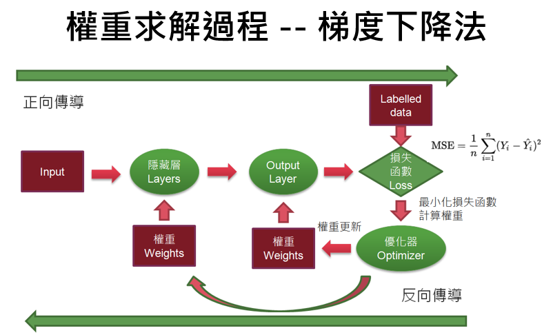

圖一. 梯度下降法的權重求解過程

不使用 model.fit而改用自動微分，可以掌控模型訓練的過程，也可以取得更多的資訊，例如：

1. 訓練過程中梯度、權重及學習率的變化。
2. 訓練過程中，可顯示模型或重建影像，類似生成式AI工具，輸入提示後，生成圖像會逐漸成形。

像PyTorch、Jax...等深度學習套件就不支援model.fit，強制開發者必須要依圖一流程，訓練模型。

實作

範例1. 自動微分測試，對y=x²自動微分。

1. 載入套件。

import tensorflow as tf 

2. 在 tf.GradientTape 中定義損失函數，使用 g.gradient 取得梯度，使用numpy()轉為NumPy格式。

x = tf.Variable(3.0)         # 宣告 TensorFlow 變數(Variable)
with tf.GradientTape() as g: # 自動微分
    y = x * x                # 損失函數
    
dy_dx = g.gradient(y, x)     # 取得梯度， f'(x) = 2x, x=3 ==> 6
print(dy_dx.numpy())         # 轉換為 NumPy array 格式

3. 將以上程式碼另存為 06_自動微分.py。
4. 執行：python 06_自動微分.py。
5. 執行結果：6.0，因為x²的一階導數為2x，第一行程式定義x=3，帶入2x = 2*3 = 6。
6. 就算定義很複雜損失函數，深度學習套件也可以幫我們算出來。例如加上三角函數sin：

x = tf.Variable(3.0)         # 宣告 TensorFlow 變數(Variable)
with tf.GradientTape() as g: # 自動微分
    y = x * tf.sin(x) ** 2   # 損失函數
    
dy_dx = g.gradient(y, x)     # 取得梯度， f'(x) = 2x, x=3 ==> 6
print(dy_dx.numpy())         # 轉換為 NumPy array 格式

7. 執行結果：-0.81833154。

範例2. 再測試 PyTorch 深度學習套件的自動微分功能，同樣對y=x²自動微分。

1. 載入套件。

import torch

2. PyTorch 不需 tf.GradientTape，直接定義損失函數，使用 g.gradient 取得梯度，使用numpy()轉為NumPy格式。

x = torch.tensor(3.0, requires_grad=True)  # 設定 x 參與自動微分
y=x*x                 # 損失函數
y.backward()          # 反向傳導
print(x.grad.numpy()) # 取得梯度

3. 將以上程式碼另存為 07_pytorch_自動微分.py。
4. 執行：python 07_pytorch_自動微分.py。
5. 執行結果也是6.0。

範例3. 以上篇為例，以自動微分對y=x²求解最小值。

1. 修改train函數：使用 tf.GradientTape 自動微分。

def train(w_start, epochs, lr):    
    w_list = np.array([])    
    w = tf.Variable(w_start)         # 宣告 TensorFlow 變數(Variable)
    w_list = np.append(w_list, w_start)  
    # 執行N個訓練週期
    for i in range(epochs):         
        with tf.GradientTape() as g: # 自動微分
            y = w * w                # 損失函數

        dw = g.gradient(y, w) # 取得梯度
        # 更新權重：新權重 = 原權重 — 學習率(learning_rate) * 梯度(gradient)
        w.assign_sub(lr * dw)  # w -=  dw * lr         
        w_list = np.append(w_list, w.numpy())    
    return w_list

2. 完整程式碼如下，可另存為 08_以自動微分實作梯度下降.py。

# 載入套件
import numpy as np
import matplotlib.pyplot as plt
from matplotlib.font_manager import FontProperties
import tensorflow as tf 

# 修正中文亂碼
plt.rcParams['font.sans-serif'] = ['Microsoft JhengHei'] 
plt.rcParams['axes.unicode_minus'] = False


# 損失函數為 y=x^2
def func(x): return x ** 2

# @tf.function
def train(w_start, epochs, lr):    
    w_list = np.array([])    
    w = tf.Variable(w_start)         # 宣告 TensorFlow 變數(Variable)
    w_list = np.append(w_list, w_start)  
    # 執行N個訓練週期
    for i in range(epochs):         
        with tf.GradientTape() as g: # 自動微分
            y = w * w                # 損失函數

        dw = g.gradient(y, w) # 取得梯度
        # 更新權重：新權重 = 原權重 — 學習率(learning_rate) * 梯度(gradient)
        w.assign_sub(lr * dw)  # w -=  dw * lr         
        w_list = np.append(w_list, w.numpy())    
    return w_list

# 模型訓練：呼叫梯度下降法 
w_start = -5.0 # 權重初始值
epochs = 150  # 訓練週期數
lr = 0.1      # 學習率
w_list = train(w_start, epochs, lr=lr) 
print (f'w:{np.around(w_list, 2)}')

# 繪圖觀察權重更新過程
color = 'r'    
t = np.arange(-6.0, 6.0, 0.01)
plt.plot(t, func(t), c='b')
plt.plot(w_list, func(w_list), c=color, label='lr={}'.format(lr))    
plt.scatter(w_list, func(w_list), c=color) 
# 繪圖箭頭，顯示權重更新方向
plt.quiver(w_list[0]-0.2, func(w_list[0]), w_list[4]-w_list[0], 
    func(w_list[4])-func(w_list[0]), color='g', scale_units='xy', scale=5)

# 繪圖標題設定
font = {'family': 'Microsoft JhengHei', 'weight': 'normal', 'size': 20}
plt.title('梯度下降法', fontproperties=font)
plt.xlabel('w', fontsize=20)
plt.ylabel('Loss', fontsize=20)
plt.show()

3. 執行：python 08_以自動微分實作梯度下降.py。
4. 執行結果與上一篇相同。
5. train函數還可以改成運算圖(@tf.function)，加速執行速度，這部分就留給讀者自行發揮了。

一元線性迴歸實作

上面範例只考慮w，若加上偏差項b，即 y = wx + b，要如何實作呢?

範例3. 一元線性迴歸。

1. 載入套件。

import matplotlib.pyplot as plt
from matplotlib.pyplot import figure
from sklearn.datasets import make_regression
import numpy as np
import tensorflow as tf 

2. 生成亂數資料。

X1, y= make_regression(n_samples=100, n_features=1, noise=15, bias=50)
X=X1.ravel() # 轉為一維陣列

3. 設定圖形屬性：我們要將訓練過程以動畫呈現。

# 設定圖形更新的頻率
PAUSE_INTERVAL=0.5

# 設定圖形大小
fig, ax = plt.subplots()
fig.set_size_inches(10, 6)
          
# 繪製亂數資料散佈圖
plt.scatter(X,y)
line, = ax.plot(X, [0] * len(X), 'r')

4. 設定MSE計算公式，即∑(y-ŷ)**2/n)。

# 求預測值(ŷ)
def predict(X):
    return w * X + b  

# 計算損失函數 MSE = ∑(y-ŷ)**2/n
def loss(y, y_pred):
    return tf.reduce_mean(tf.square(y - y_pred))

5. 定義繪製迴歸線的函數。

def draw(w, b):
    # 更新圖形Y軸資料
    y_new = [b + w * xplot for xplot in X]
    line.set_data(X, y_new)  # update the data.
    #ax.cla()
    plt.pause(PAUSE_INTERVAL)

6. 定義訓練函數：損失函數對w、b各自偏微分，w、b也獨立更新。

def train(X, y, epochs=40, lr=0.1):
    current_loss=0                                # 損失函數值
    for epoch in range(epochs):                   # 執行訓練週期
        with tf.GradientTape() as t:              # 自動微分
            t.watch(tf.constant(X))               # 宣告 TensorFlow 常數參與自動微分
            current_loss = loss(y, predict(X))    # 計算損失函數值
        
        dw, db = t.gradient(current_loss, [w, b]) # 取得 w, b 個別的梯度

        # 更新權重：新權重 = 原權重 — 學習率(learning_rate) * 梯度(gradient)
        w.assign_sub(lr * dw) # w -= lr * dw
        b.assign_sub(lr * db) # b -= lr * db
        
        # 更新圖形
        draw(w, b)
        
        # 顯示每一訓練週期的損失函數
        print(f'Epoch {epoch}: Loss: {current_loss.numpy()}') 

7. 模型訓練。

# w、b 初始值均設為 0
w = tf.Variable(0.0)
b = tf.Variable(0.0)

# 執行訓練
train(X, y)

8. 驗證 w、b是否正確：使用Scikit-learn套件比對。

from sklearn.metrics import mean_squared_error
from sklearn.linear_model import LinearRegression
model = LinearRegression()
model.fit(X1, y)
print(f'w={model.coef_[0]}, b={model.intercept_}')

9. 完整程式碼如下，可另存為 10_簡單線性迴歸_自動微分.py。

# 載入套件
import matplotlib.pyplot as plt
from matplotlib.pyplot import figure
from sklearn.datasets import make_regression
import numpy as np
import tensorflow as tf 

# 生成亂數資料
X1, y= make_regression(n_samples=100, n_features=1, noise=15, bias=50)
X=X1.ravel() # 轉為一維陣列
# print(X, y)  

# 設定圖形更新的頻率
PAUSE_INTERVAL=0.5

# 設定圖形大小
fig, ax = plt.subplots()
fig.set_size_inches(10, 6)
          
# 繪製亂數資料散佈圖
plt.scatter(X,y)
line, = ax.plot(X, [0] * len(X), 'r')

# 求預測值(Y hat)
def predict(X):
    return w * X + b  

# 計算損失函數 MSE = ∑(y-ŷ)**2/n
def loss(y, y_pred):
    return tf.reduce_mean(tf.square(y - y_pred))

# 定義繪製迴歸線的函數
def draw(w, b):
    # 更新圖形Y軸資料
    y_new = [b + w * xplot for xplot in X]
    line.set_data(X, y_new)  # update the data.
    #ax.cla()
    plt.pause(PAUSE_INTERVAL)

# 定義訓練函數
def train(X, y, epochs=40, lr=0.1):
    current_loss=0                                # 損失函數值
    for epoch in range(epochs):                   # 執行訓練週期
        with tf.GradientTape() as t:              # 自動微分
            t.watch(tf.constant(X))               # 宣告 TensorFlow 常數參與自動微分
            current_loss = loss(y, predict(X))    # 計算損失函數值
        
        dw, db = t.gradient(current_loss, [w, b]) # 取得 w, b 個別的梯度

        # 更新權重：新權重 = 原權重 — 學習率(learning_rate) * 梯度(gradient)
        w.assign_sub(lr * dw) # w -= lr * dw
        b.assign_sub(lr * db) # b -= lr * db
        
        # 更新圖形
        draw(w, b)
        
        # 顯示每一訓練週期的損失函數
        print(f'Epoch {epoch}: Loss: {current_loss.numpy()}') 

# 模型訓練        
# w、b 初始值均設為 0
w = tf.Variable(0.0)
b = tf.Variable(0.0)

# 執行訓練
train(X, y)

# w、b 的最佳解
print(f'w={w.numpy()}, b={b.numpy()}')

# 顯示動畫       
# plt.show()

# 驗證 w、b是否正確：使用Scikit-learn套件比對
from sklearn.metrics import mean_squared_error
from sklearn.linear_model import LinearRegression
model = LinearRegression()
model.fit(X1, y)
print(f'w={model.coef_[0]}, b={model.intercept_}')

10. 執行：python 10_簡單線性迴歸_自動微分.py。

11. 執行結果：w、b逐步更新，最終迴歸線自亂數資料中間穿過。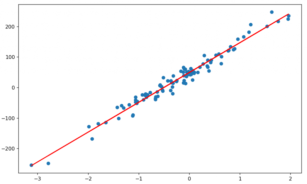
    

12. 驗證 w、b：與Scikit-learn套件計算結果非常相近。

梯度下降法：w=87.38388061523438, b=48.79069519042969
Scikit-learn：w=87.39229369, b=48.788610878339966

13. 多元線性迴歸實作，只要修改亂數資料生成的參數 n_features=特徵個數，同時訓練時以迴圈處理多個w自動為分及更新。

X, y= make_regression(n_samples=100, n_features=2, noise=15, bias=50)

結語

本篇介紹以自動微分(Automatic Differentiation)實作梯度下降，下一篇我們介紹一些應用，不限於神經網路：

1. 以自動微分實作手寫阿拉伯數字辨識，結合Keras模型，兼顧程式簡潔與彈性。
2. 聯立方程式求解。
3. 機器學習演算法，例如羅吉斯迴歸(Logistic regression)、支援向量機(Support vector machine，SVM)...等。

Happy coding !!

工商廣告:)

《深度學習最佳入門與專題實戰》導讀講座 2025/07/11 歡迎報名

書籍：

1. 深度學習最佳入門與專題實戰：理論基礎與影像篇, 2025/05 再版
2. 深度學習最佳入門與專題實戰：自然語言處理、大型語言模型與強化學習篇, 2025/05 再版
3. 開發者傳授 PyTorch 秘笈
4. Scikit-learn 詳解與企業應用

影音課程：

深度學習PyTorch入門到實戰應用

企業包班

系列文章目錄

徹底理解神經網路的核心 -- 梯度下降法 (1)
徹底理解神經網路的核心 -- 梯度下降法 (2)
徹底理解神經網路的核心 -- 梯度下降法 (3)
徹底理解神經網路的核心 -- 梯度下降法 (4)
徹底理解神經網路的核心 -- 梯度下降法 (5)