魔鬼藏在細節裡，要讓模型訓練更快速、更準確，必須進一步掌握模型的超參數(Hyperparameters)設定，包括如何動態調整學習率、選用各種優化器、損失函數、Activation function...等，本篇先探討學習率的調整，並尋找最佳學習率初始值。

註：超參數(Hyperparameters)是指模型訓練前可以調整的參數，例如權重初始值、學習率、執行週期，如以程式角度而言，優化器、損失函數、Activation function也都是函數的參數，而一般參數通常指的是模型的權重(Weight)與偏差(Bias)。

學習率

如下圖，反向傳導會使用優化器(Optimizer)更新權重，公式如下：
新權重 = 原權重 — 學習率(learning rate) * 梯度(gradient)
在前幾篇我們都設定學習率為固定值，更好的方法是動態調整學習率，訓練一開始，離最佳解很遠時，可設定較大的學習率，快步前進，之後逐步縮小，避免錯過最佳解，並找到更精準的解。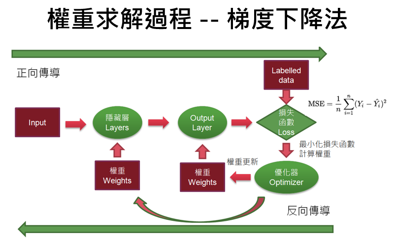

圖一. 梯度下降法的權重求解過程

範例1. 動態調整學習率，加速簡單損失函數求解。

1. 修改第三篇05_函數的梯度下降.py的train函數，加倒數第二行，學習率每週期減少1/100。

def train(w_start, epochs, lr):    
    w_list = np.zeros(epochs+1)    
    w = w_start    
    w_list[0] = w  
    # 執行N個訓練週期
    for i in range(epochs):         
        # 權重的更新W_new
        # W_new = W — learning_rate * gradient        
        w -=  dfunc(w) * lr         
        w_list[i+1] = w    
        lr -= lr/100 # 學習率每週期減少1/100
    return w_list

2. 初始學習率從0.1加大為0.2。

lr = 0.2     # 學習率

3. 另存為 15_函數的梯度下降_動態調整學習率.py。
4. 執行：python 15_函數的梯度下降_動態調整學習率.py。
5. 執行結果：原來要32個訓練週期才收斂，現在只要15個週期就收斂了，確實可縮短求解時間。
   

TensorFlow 實作

如何在TensorFlow中動態調整學習率呢? 請看下列範例。
範例2. 動態調整學習率與取得學習率。

1. 載入套件。

import tensorflow as tf
import numpy as np
import matplotlib.pyplot as plt

2. 定義函數在訓練過程中顯示學習率：須在函數內定義lr函數。

def get_lr_metric(optimizer):
    def lr(y_true, y_pred):
        return optimizer._get_current_learning_rate()
    return lr

3. 模型定義：最後兩行生成get_lr_metric物件，並在model.compile內額外顯示物件。

model = tf.keras.models.Sequential([tf.keras.layers.Input((20,)), tf.keras.layers.Dense(10)])
optimizer = tf.keras.optimizers.Adam()
lr_metric = get_lr_metric(optimizer)
model.compile(optimizer, loss='sparse_categorical_crossentropy', metrics=['accuracy', lr_metric])

4. 動態調整學習率：設定前 10 個訓練週期的學習率為固定值，之後逐次衰減。

def scheduler(epoch, lr):
    if epoch < 10:
        return lr
    else:
        return np.float64(lr * tf.math.exp(-0.1)) # 學習率每週期約減少1/10

5. 在 Callback 中呼叫scheduler改變學習率。

callback = tf.keras.callbacks.LearningRateScheduler(scheduler)

6. 模型訓練：使用亂數作為訓練資料，因為我們只是要測試動態調整學習率。

history = model.fit(np.arange(100).reshape(5, 20), np.zeros(5),
                    epochs=15, callbacks=[callback], verbose=2)

7. 對訓練過程的學習率繪圖。

plt.figure(figsize=(8, 6))
plt.plot(history.history['lr'], 'r')
plt.show()

8. 完整程式碼如下，另存為 16_Get_learning_rate.py。

9. 執行：python 16_Get_learning_rate.py。

10. 執行結果：後5個週期逐次減少1/10。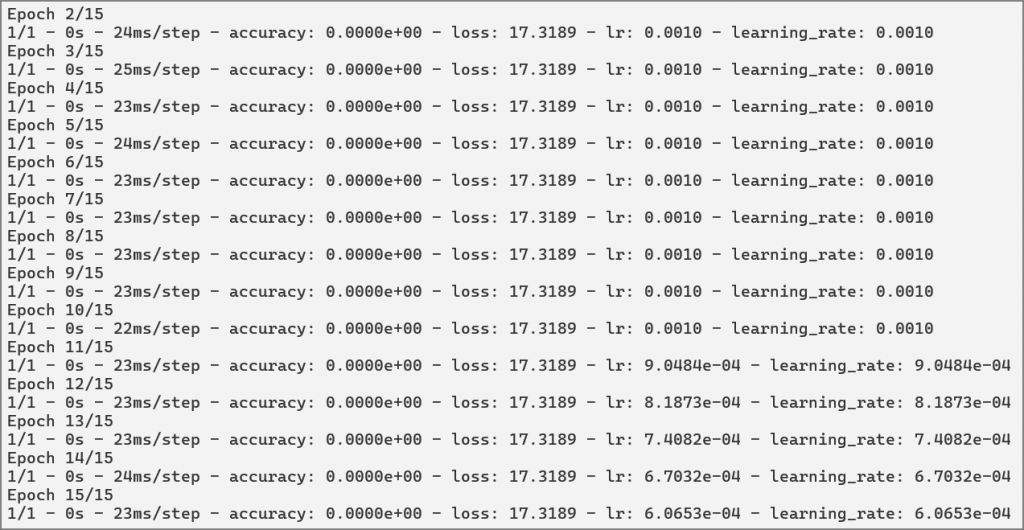
    

11. 繪圖。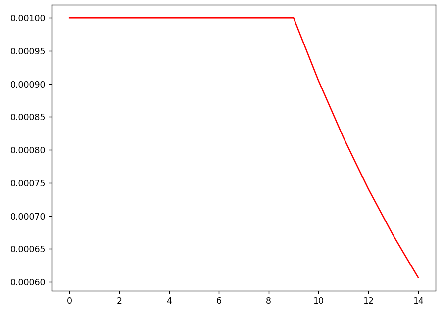
    

尋找最佳學習率初始值

知道如何動態調整學習率後，那學習率初始值要設多少呢?

範例3. 動態調整學習率與取得學習率。

1. 載入套件：最後一行呼叫lr_finder.py，它定義尋找最佳學習率初始值的方法。

import tensorflow as tf
from tensorflow.keras.layers import Conv2D, MaxPool2D, Flatten, Dense, Dropout
import matplotlib.pyplot as plt
from lr_finder import LRFinder

2. 載入訓練資料：使用Fashion MNIST，它含10類的女士配件。

fashion_mnist = tf.keras.datasets.fashion_mnist
(x_train, y_train), (x_valid, y_valid) = fashion_mnist.load_data()
x_train, x_valid = x_train / 255.0, x_valid / 255.0
x_train = x_train[..., tf.newaxis]
x_valid = x_valid[..., tf.newaxis]
train_ds = tf.data.Dataset.from_tensor_slices((x_train, y_train)).shuffle(10000).batch(32)
valid_ds = tf.data.Dataset.from_tensor_slices((x_valid, y_valid)).batch(32)

3. 模型定義。

def build_model():
    return tf.keras.models.Sequential([
        Conv2D(32, 3, activation='relu'),
        MaxPool2D(),
        Flatten(),
        Dense(128, activation='relu'),
        Dropout(0.1),
        Dense(10, activation='softmax')
    ])

4. 模型訓練：callback加上lr_finder。

lr_finder = LRFinder()
model = build_model()
adam = tf.keras.optimizers.Adam(learning_rate=1e-1)
model.compile(optimizer=adam, loss='sparse_categorical_crossentropy', metrics=['accuracy'])
model.fit(train_ds, epochs=5, callbacks=[lr_finder])

5. 對訓練過程的學習率繪圖。

lr_finder.plot()
plt.axvline(1e-3, c='r');
plt.show()

6. 模型評分。

_, accuracy = model.evaluate(valid_ds, verbose=False)
print(f'accuracy={accuracy}')

7. 採用使最佳學習率重新訓練。

model = build_model() # reinitialize model
adam = tf.optimizers.Adam(1e-3)
model.compile(optimizer=adam, loss='sparse_categorical_crossentropy', metrics=['accuracy'])
_ = model.fit(train_ds, validation_data=valid_ds, epochs=5, verbose=True)
_, accuracy = model.evaluate(valid_ds, verbose=False)
print(f'最佳學習率 accuracy={accuracy}')

8. 完整程式碼如下，另存為 17_tf_lr_finder.py。

# 尋找最佳學習率初始值

# 載入套件
import tensorflow as tf
from tensorflow.keras.layers import Conv2D, MaxPool2D, Flatten, Dense, Dropout
import matplotlib.pyplot as plt
from lr_finder import LRFinder

# 載入訓練資料
fashion_mnist = tf.keras.datasets.fashion_mnist
(x_train, y_train), (x_valid, y_valid) = fashion_mnist.load_data()
x_train, x_valid = x_train / 255.0, x_valid / 255.0
x_train = x_train[..., tf.newaxis]
x_valid = x_valid[..., tf.newaxis]
train_ds = tf.data.Dataset.from_tensor_slices((x_train, y_train)).shuffle(10000).batch(32)
valid_ds = tf.data.Dataset.from_tensor_slices((x_valid, y_valid)).batch(32)

# 模型定義
def build_model():
    return tf.keras.models.Sequential([
        Conv2D(32, 3, activation='relu'),
        MaxPool2D(),
        Flatten(),
        Dense(128, activation='relu'),
        Dropout(0.1),
        Dense(10, activation='softmax')
    ])

# 模型訓練
lr_finder = LRFinder()
model = build_model()
adam = tf.keras.optimizers.Adam(learning_rate=1e-1)
model.compile(optimizer=adam, loss='sparse_categorical_crossentropy', metrics=['accuracy'])
model.fit(train_ds, epochs=5, callbacks=[lr_finder])

# 對訓練過程的學習率繪圖
lr_finder.plot()
plt.axvline(1e-3, c='r');
plt.show()

# 模型評分
_, accuracy = model.evaluate(valid_ds, verbose=False)
print(f'accuracy={accuracy}')


# 採用最佳學習率重新訓練。
model = build_model() # reinitialize model
adam = tf.optimizers.Adam(1e-3)
model.compile(optimizer=adam, loss='sparse_categorical_crossentropy', metrics=['accuracy'])
_ = model.fit(train_ds, validation_data=valid_ds, epochs=5, verbose=True)
_, accuracy = model.evaluate(valid_ds, verbose=False)
print(f'最佳學習率 accuracy={accuracy}')

9. 另外，lr_finder.py完整程式碼如下，可詳閱『How Do You Find A Good Learning Rate』，它採取指數退火(Exponential annealing)動態調整學習率。

import matplotlib.pyplot as plt
import tensorflow as tf

from tensorflow.keras.callbacks import Callback


class LRFinder(Callback):
    """`Callback` that exponentially adjusts the learning rate after each training batch between `start_lr` and
    `end_lr` for a maximum number of batches: `max_step`. The loss and learning rate are recorded at each step allowing
    visually finding a good learning rate as per https://sgugger.github.io/how-do-you-find-a-good-learning-rate.html via
    the `plot` method.
    """

    def __init__(self, start_lr: float = 1e-7, end_lr: float = 10, max_steps: int = 100, smoothing=0.9):
        super(LRFinder, self).__init__()
        self.start_lr, self.end_lr = start_lr, end_lr
        self.max_steps = max_steps
        self.smoothing = smoothing
        self.step, self.best_loss, self.avg_loss, self.lr = 0, 0, 0, 0
        self.lrs, self.losses = [], []

    def on_train_begin(self, logs=None):
        self.step, self.best_loss, self.avg_loss, self.lr = 0, 0, 0, 0
        self.lrs, self.losses = [], []

    def on_train_batch_begin(self, batch, logs=None):
        self.lr = self.exp_annealing(self.step)
        self.model.optimizer.learning_rate=self.lr

    def on_train_batch_end(self, batch, logs=None):
        logs = logs or {}
        loss = logs.get('loss')
        step = self.step
        if loss:
            self.avg_loss = self.smoothing * self.avg_loss + (1 - self.smoothing) * loss
            smooth_loss = self.avg_loss / (1 - self.smoothing ** (self.step + 1))
            self.losses.append(smooth_loss)
            self.lrs.append(self.lr)

            if step == 0 or loss < self.best_loss:
                self.best_loss = loss

            if smooth_loss > 4 * self.best_loss or tf.math.is_nan(smooth_loss):
                self.model.stop_training = True

        if step == self.max_steps:
            self.model.stop_training = True

        self.step += 1

    def exp_annealing(self, step):
        return self.start_lr * (self.end_lr / self.start_lr) ** (step * 1. / self.max_steps)

    def plot(self):
        fig, ax = plt.subplots(1, 1)
        ax.set_ylabel('Loss')
        ax.set_xlabel('Learning Rate (log scale)')
        ax.set_xscale('log')
        ax.xaxis.set_major_formatter(plt.FormatStrFormatter('%.0e'))
        ax.plot(self.lrs, self.losses)

10. 執行：python 17_tf_lr_finder.py。

11. 執行結果：最佳學習率為10**-3，該點以前損失減少的幅度非常小，從10**-3開始可以有效地降低損失。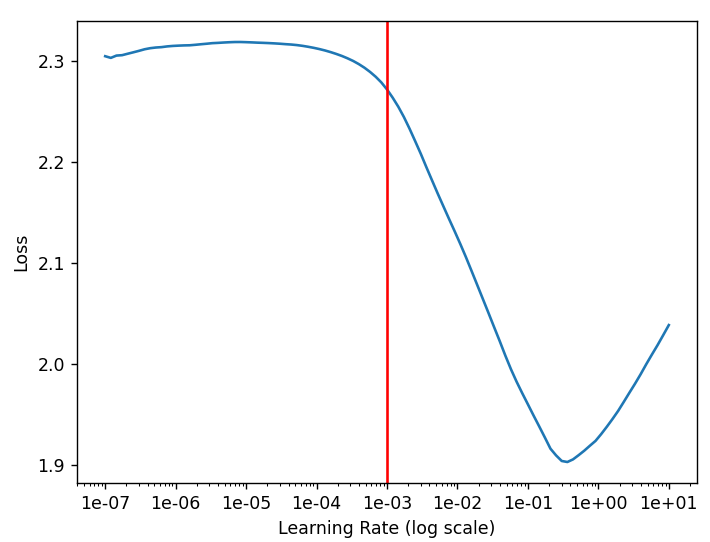
    

12. 使用動態調整學習率的模型訓練與採用最佳學習率(10**-3)重新訓練結果相同，表示lr_finder.py確實可以找到最佳學習率初始值。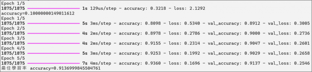
    

結語

動態調整學習率可以很複雜，不僅讓模型訓練更快速、更準確，也希望避開區域最小值(Local minimum)，找尋全局最小值(Global minimum)，有興趣的讀者可參閱『A Gentle Introduction to Learning Rate Schedulers』及相關論文。

工商廣告:)

《深度學習最佳入門與專題實戰》導讀講座 2025/07/11 歡迎報名

書籍：

1. 深度學習最佳入門與專題實戰：理論基礎與影像篇, 2025/05 再版
2. 深度學習最佳入門與專題實戰：自然語言處理、大型語言模型與強化學習篇, 2025/05 再版
3. 開發者傳授 PyTorch 秘笈
4. Scikit-learn 詳解與企業應用

影音課程：

深度學習PyTorch入門到實戰應用

企業包班

系列文章目錄

徹底理解神經網路的核心 -- 梯度下降法 (1)
徹底理解神經網路的核心 -- 梯度下降法 (2)
徹底理解神經網路的核心 -- 梯度下降法 (3)
徹底理解神經網路的核心 -- 梯度下降法 (4)
徹底理解神經網路的核心 -- 梯度下降法的應用 (5)
梯度下降法(6) -- 學習率動態調整
梯度下降法(7) -- 優化器(Optimizer)