到今天為止,我們已經理解大部分 CNN 的基本概念(卷積、池化等)。
在學習完後馬上開始實作我覺得是最適合不過的了,把「理論」變成「可以跑起來的模型」。
今天我們會用 Keras(TensorFlow)從零建立一個簡單但完整的 CNN,
訓練它去分類 CIFAR-10 的圖片,並展示訓練、評估與推論流程。
由於此文章篇幅較長,我會將該篇文章拆成兩天上傳,還請讀者見諒。
那我們就馬上開始吧!!!
(程式碼可直接在 Colab 或本地有 GPU 的環境執行)
首先我們先來了解一下這個實作要做什麼,
我們主要會將其分為以下幾個步驟:
以上就是我們今天要一步步實作的幾個目標內容,接著就進到程式碼:
首先我們就先把全部的程式碼先呈現出來給各位,稍後再做講解:
import tensorflow as tf
from tensorflow.keras import layers, models
from tensorflow.keras.preprocessing.image import ImageDataGenerator
import matplotlib.pyplot as plt
import numpy as np
import os

# 設定隨機種子以確保可重現性
tf.random.set_seed(42)
np.random.seed(42)

# CIFAR-10 類別名稱
class_names = ['airplane', 'automobile', 'bird', 'cat', 'deer',
               'dog', 'frog', 'horse', 'ship', 'truck']

# 1. 載入並檢查資料
print("載入 CIFAR-10 資料...")
(x_train, y_train), (x_test, y_test) = tf.keras.datasets.cifar10.load_data()
y_train = y_train.reshape(-1)
y_test = y_test.reshape(-1)

print(f"訓練集形狀: {x_train.shape}, 標籤: {y_train.shape}")
print(f"測試集形狀: {x_test.shape}, 標籤: {y_test.shape}")
print(f"像素值範圍: [{x_train.min()}, {x_train.max()}]")

# 2. 改進的資料前處理
def preprocess_data(x_train, x_test, y_train, y_test):
    # 正規化到 [0,1]
    x_train = x_train.astype('float32') / 255.0
    x_test = x_test.astype('float32') / 255.0

    # 可選:標準化 (zero-mean, unit variance)
    # mean = x_train.mean(axis=(0,1,2), keepdims=True)
    # std = x_train.std(axis=(0,1,2), keepdims=True)
    # x_train = (x_train - mean) / (std + 1e-7)
    # x_test = (x_test - mean) / (std + 1e-7)

    return x_train, x_test, y_train, y_test

x_train, x_test, y_train, y_test = preprocess_data(x_train, x_test, y_train, y_test)

# 3. 改進的 CNN 模型架構
def build_improved_cnn(input_shape=(32, 32, 3), num_classes=10, dropout_rate=0.3):
    inputs = layers.Input(shape=input_shape)

    # Block 1: 淺層特徵
    x = layers.Conv2D(32, (3,3), padding='same', kernel_initializer='he_normal')(inputs)
    x = layers.BatchNormalization()(x)
    x = layers.ReLU()(x)
    x = layers.Conv2D(32, (3,3), padding='same', kernel_initializer='he_normal')(x)
    x = layers.BatchNormalization()(x)
    x = layers.ReLU()(x)
    x = layers.MaxPooling2D((2,2))(x)
    x = layers.Dropout(dropout_rate * 0.8)(x)  # 較低的 dropout

    # Block 2: 中層特徵
    x = layers.Conv2D(64, (3,3), padding='same', kernel_initializer='he_normal')(x)
    x = layers.BatchNormalization()(x)
    x = layers.ReLU()(x)
    x = layers.Conv2D(64, (3,3), padding='same', kernel_initializer='he_normal')(x)
    x = layers.BatchNormalization()(x)
    x = layers.ReLU()(x)
    x = layers.MaxPooling2D((2,2))(x)
    x = layers.Dropout(dropout_rate)(x)

    # Block 3: 深層特徵 (新增)
    x = layers.Conv2D(128, (3,3), padding='same', kernel_initializer='he_normal')(x)
    x = layers.BatchNormalization()(x)
    x = layers.ReLU()(x)
    x = layers.Conv2D(128, (3,3), padding='same', kernel_initializer='he_normal')(x)
    x = layers.BatchNormalization()(x)
    x = layers.ReLU()(x)
    x = layers.MaxPooling2D((2,2))(x)
    x = layers.Dropout(dropout_rate)(x)

    # Global Average Pooling 替代部分全連接層
    x = layers.GlobalAveragePooling2D()(x)

    # 分類層
    x = layers.Dense(256, kernel_regularizer=tf.keras.regularizers.l2(1e-4))(x)
    x = layers.BatchNormalization()(x)
    x = layers.ReLU()(x)
    x = layers.Dropout(dropout_rate * 1.5)(x)  # 較高的 dropout

    outputs = layers.Dense(num_classes, activation='softmax')(x)

    return models.Model(inputs, outputs, name='ImprovedCNN')

# 建立模型
model = build_improved_cnn()
model.summary()

# 4. 改進的編譯配置
# 使用 cosine decay 學習率調度
initial_learning_rate = 1e-3
lr_schedule = tf.keras.optimizers.schedules.CosineDecay(
    initial_learning_rate,
    decay_steps=1000,  # 會在訓練過程中調整
    alpha=1e-6
)

model.compile(
    optimizer=tf.keras.optimizers.Adam(learning_rate=lr_schedule),
    loss='sparse_categorical_crossentropy',
    metrics=['accuracy', tf.keras.metrics.SparseTopKCategoricalAccuracy(k=5, name='top_5_accuracy')]
)

# 5. 更豐富的資料增強
train_datagen = ImageDataGenerator(
    rotation_range=20,
    width_shift_range=0.2,
    height_shift_range=0.2,
    shear_range=0.2,
    zoom_range=0.2,
    horizontal_flip=True,
    fill_mode='nearest'
)

# 驗證集不使用資料增強
val_datagen = ImageDataGenerator()

train_datagen.fit(x_train)

# 6. 改進的 callbacks
def create_callbacks():
    return [
        tf.keras.callbacks.ModelCheckpoint(
            'best_cifar10_model.h5',
            monitor='val_accuracy',
            save_best_only=True,
            save_weights_only=False,
            verbose=1
        ),
        tf.keras.callbacks.ReduceLROnPlateau(
            monitor='val_loss',
            factor=0.3,
            patience=5,
            min_lr=1e-7,
            verbose=1
        ),
        tf.keras.callbacks.EarlyStopping(
            monitor='val_loss',
            patience=15,
            restore_best_weights=True,
            verbose=1
        ),
        tf.keras.callbacks.CSVLogger('training_log.csv')
    ]

callbacks = create_callbacks()

# 7. 訓練模型
batch_size = 128
epochs = 100

print("開始訓練...")
history = model.fit(
    train_datagen.flow(x_train, y_train, batch_size=batch_size),
    steps_per_epoch=len(x_train) // batch_size,
    epochs=epochs,
    validation_data=(x_test, y_test),
    callbacks=callbacks,
    verbose=1  # 改為 1 以看到進度條
)

# 8. 詳細評估
def evaluate_model(model, x_test, y_test):
    print("\n=== 模型評估 ===")
    results = model.evaluate(x_test, y_test, verbose=0)

    # 處理不同數量的指標
    if isinstance(results, list):
        test_loss = results[0]
        test_acc = results[1]
        if len(results) > 2:
            test_top5 = results[2]
            print(f"測試集損失值: {test_loss:.4f}")
            print(f"測試集正確率: {test_acc:.4f} ({test_acc*100:.2f}%)")
            print(f"Top-5 正確率: {test_top5:.4f} ({test_top5*100:.2f}%)")
        else:
            print(f"測試集損失值: {test_loss:.4f}")
            print(f"測試集正確率: {test_acc:.4f} ({test_acc*100:.2f}%)")
    else:
        # 只有一個值的情況
        test_loss = results
        test_acc = 0.0
        print(f"測試集損失值: {test_loss:.4f}")

    # 預測並計算混淆矩陣
    y_pred = model.predict(x_test, verbose=0)
    y_pred_classes = np.argmax(y_pred, axis=1)

    return test_acc, y_pred_classes

test_acc, y_pred_classes = evaluate_model(model, x_test, y_test)

# 9. 改進的視覺化
def plot_training_history(history):
    fig, axes = plt.subplots(2, 2, figsize=(15, 10))

    # Loss 曲線
    axes[0,0].plot(history.history['loss'], label='訓練 Loss', linewidth=2)
    axes[0,0].plot(history.history['val_loss'], label='驗證 Loss', linewidth=2)
    axes[0,0].set_title('Loss 曲線', fontsize=14)
    axes[0,0].set_xlabel('Epoch')
    axes[0,0].set_ylabel('Loss')
    axes[0,0].legend()
    axes[0,0].grid(True, alpha=0.3)

    # Accuracy 曲線
    axes[0,1].plot(history.history['accuracy'], label='訓練 Accuracy', linewidth=2)
    axes[0,1].plot(history.history['val_accuracy'], label='驗證 Accuracy', linewidth=2)
    axes[0,1].set_title('Accuracy 曲線', fontsize=14)
    axes[0,1].set_xlabel('Epoch')
    axes[0,1].set_ylabel('Accuracy')
    axes[0,1].legend()
    axes[0,1].grid(True, alpha=0.3)

    # Learning Rate 曲線 (如果有記錄)
    if 'lr' in history.history:
        axes[1,0].plot(history.history['lr'], linewidth=2, color='orange')
        axes[1,0].set_title('Learning Rate', fontsize=14)
        axes[1,0].set_xlabel('Epoch')
        axes[1,0].set_ylabel('Learning Rate')
        axes[1,0].set_yscale('log')
        axes[1,0].grid(True, alpha=0.3)

    # Top-5 Accuracy
    if 'top_5_accuracy' in history.history:
        axes[1,1].plot(history.history['top_5_accuracy'], label='訓練 Top-5', linewidth=2)
        axes[1,1].plot(history.history['val_top_5_accuracy'], label='驗證 Top-5', linewidth=2)
        axes[1,1].set_title('Top-5 Accuracy 曲線', fontsize=14)
        axes[1,1].set_xlabel('Epoch')
        axes[1,1].set_ylabel('Top-5 Accuracy')
        axes[1,1].legend()
        axes[1,1].grid(True, alpha=0.3)

    plt.tight_layout()
    plt.savefig('training_curves.png', dpi=300, bbox_inches='tight')
    plt.show()

plot_training_history(history)

# 10. 改進的預測展示
def show_predictions(model, x_test, y_test, num_samples=8):
    """展示預測結果和真實標籤"""
    fig, axes = plt.subplots(2, 4, figsize=(16, 8))
    axes = axes.ravel()

    # 隨機選擇樣本
    indices = np.random.choice(len(x_test), num_samples, replace=False)

    for i, idx in enumerate(indices):
        img = x_test[idx]
        pred = model.predict(img[np.newaxis, ...], verbose=0)
        pred_class = np.argmax(pred[0])
        pred_prob = np.max(pred[0])
        true_class = y_test[idx]

        axes[i].imshow(img)
        axes[i].axis('off')

        # 設定顏色:正確=綠色,錯誤=紅色
        color = 'green' if pred_class == true_class else 'red'
        axes[i].set_title(
            f'True: {class_names[true_class]}\n'
            f'Pred: {class_names[pred_class]}\n'
            f'Conf: {pred_prob:.3f}',
            color=color, fontsize=10
        )

    plt.tight_layout()
    plt.savefig('predictions_sample.png', dpi=300, bbox_inches='tight')
    plt.show()

show_predictions(model, x_test, y_test)

# 11. 模型儲存
print("\n儲存最終模型...")
model.save('cifar10_improved_cnn.h5')
print("模型已儲存為 'cifar10_improved_cnn.h5'")

# 12. 儲存訓練歷史
import pickle
with open('training_history.pkl', 'wb') as f:
    pickle.dump(history.history, f)
print("訓練歷史已儲存為 'training_history.pkl'")

# 輸出最終結果摘要
print(f"\n=== 訓練完成 ===")
print(f"最佳驗證準確率: {max(history.history['val_accuracy']):.4f}")
print(f"最終測試準確率: {test_acc:.4f}")
print(f"訓練總輪數: {len(history.history['loss'])}")
我也在程式碼中加入了段落註解,接著我們就根據段落一個一個來看,
如果在閱讀中有特別想了解的部分,
也可以根據註解直接拉到該段落的解釋。
import tensorflow as tf
from tensorflow.keras import layers, models
from tensorflow.keras.preprocessing.image import ImageDataGenerator
import matplotlib.pyplot as plt
import numpy as np
import os

# 設定隨機種子以確保可重現性
tf.random.set_seed(42)
np.random.seed(42)

# CIFAR-10 類別名稱
class_names = ['airplane', 'automobile', 'bird', 'cat', 'deer',
               'dog', 'frog', 'horse', 'ship', 'truck']
首先我們要準備工作環境,就像廚師做菜前要準備所有的工具和材料一樣。
我們匯入所有必要的套件:TensorFlow 是我們的主要深度學習框架,
matplotlib 用於畫圖和視覺化,numpy 則是處理數值計算。
特別重要的是「設定隨機種子」。電腦在訓練過程中會產生很多隨機數字,
設定種子就像固定骰子的點數一樣,確保每次執行程式時都能得到相同的結果。
這對於科學實驗的可重現性非常重要,
如果今天訓練得到 90% 準確率,明天重跑一次也應該得到類似的結果。
我們也預先定義了 CIFAR-10 的 10 個類別名稱,這樣當電腦預測出數字時,
我們就可以根據他顯示的數字判斷出是什麼圖片(0-9,共10個)。
# 載入並檢查資料
print("載入 CIFAR-10 資料...")
(x_train, y_train), (x_test, y_test) = tf.keras.datasets.cifar10.load_data()
y_train = y_train.reshape(-1)
y_test = y_test.reshape(-1)

print(f"訓練集形狀: {x_train.shape}, 標籤: {y_train.shape}")
print(f"測試集形狀: {x_test.shape}, 標籤: {y_test.shape}")
print(f"像素值範圍: [{x_train.min()}, {x_train.max()}]")
現在我們要載入資料,就像打開一個裝滿照片的箱子。
Keras 很貼心地提供了方便的 API 來載入 CIFAR-10 資料集,
不用我們自己去網路上下載和整理。
資料則會自動分為兩部分:
訓練集(50,000 張圖片)和測試集(10,000 張圖片)。
這就像準備考試一樣,用訓練集來「讀書學習」,測試集則用來「模擬考試」。
原始的標籤是二維陣列(像是一個表格),
我們使用 reshape(-1) 把它變成一條直線(一維陣列),這樣在後續處理時比較方便。
透過印出資料形狀,我們可以確認資料的基本資訊:
-訓練集:50,000 張 32x32x3 的彩色圖片(3 代表紅綠藍三個顏色通道)
-測試集:10,000 張圖片
-像素值範圍:0-255(還沒有經過處理的原始狀態)
def preprocess_data(x_train, x_test, y_train, y_test):
    # 正規化到 [0,1]
    x_train = x_train.astype('float32') / 255.0
    x_test = x_test.astype('float32') / 255.0

    return x_train, x_test, y_train, y_test

x_train, x_test, y_train, y_test = preprocess_data(x_train, x_test, y_train, y_test)
再來是訓練前的資料處理。
我們將像素值從整數轉換為浮點數,並將數值範圍從 0-255 縮放到 0-1(除以255)。
這個過程叫做正規化(Normalization)。
在前面的實作中,這已經是我們必做的步驟了,這邊再講解一次:
因為 255 這種大數字在神經網路的計算中可能會造成數值不穩定,
所以我們把它們都縮小到 0-1 之間,讓所有數字都在同一個尺度上。
這樣做會有兩個好處:
-數值穩定性:較小的數值範圍讓模型在計算梯度時更穩定,不會出現數值爆炸的問題
-訓練效率:正規化後的資料能讓模型學習得更快,更容易找到最佳解
def build_improved_cnn(input_shape=(32, 32, 3), num_classes=10, dropout_rate=0.3):
    inputs = layers.Input(shape=input_shape)

    # Block 1: 淺層特徵
    x = layers.Conv2D(32, (3,3), padding='same', kernel_initializer='he_normal')(inputs)
    x = layers.BatchNormalization()(x)
    x = layers.ReLU()(x)
    x = layers.Conv2D(32, (3,3), padding='same', kernel_initializer='he_normal')(x)
    x = layers.BatchNormalization()(x)
    x = layers.ReLU()(x)
    x = layers.MaxPooling2D((2,2))(x)
    x = layers.Dropout(dropout_rate * 0.8)(x)  # 較低的 dropout

    # Block 2: 中層特徵
    x = layers.Conv2D(64, (3,3), padding='same', kernel_initializer='he_normal')(x)
    x = layers.BatchNormalization()(x)
    x = layers.ReLU()(x)
    x = layers.Conv2D(64, (3,3), padding='same', kernel_initializer='he_normal')(x)
    x = layers.BatchNormalization()(x)
    x = layers.ReLU()(x)
    x = layers.MaxPooling2D((2,2))(x)
    x = layers.Dropout(dropout_rate)(x)

    # Block 3: 深層特徵
    x = layers.Conv2D(128, (3,3), padding='same', kernel_initializer='he_normal')(x)
    x = layers.BatchNormalization()(x)
    x = layers.ReLU()(x)
    x = layers.Conv2D(128, (3,3), padding='same', kernel_initializer='he_normal')(x)
    x = layers.BatchNormalization()(x)
    x = layers.ReLU()(x)
    x = layers.MaxPooling2D((2,2))(x)
    x = layers.Dropout(dropout_rate)(x)

    # Global Average Pooling 替代部分全連接層
    x = layers.GlobalAveragePooling2D()(x)

    # 分類層
    x = layers.Dense(256, kernel_regularizer=tf.keras.regularizers.l2(1e-4))(x)
    x = layers.BatchNormalization()(x)
    x = layers.ReLU()(x)
    x = layers.Dropout(dropout_rate * 1.5)(x)  # 較高的 dropout

    outputs = layers.Dense(num_classes, activation='softmax')(x)

    return models.Model(inputs, outputs, name='ImprovedCNN')

# 建立模型
model = build_improved_cnn()
model.summary()
接著就是整個實作最核心的部分 - 設計我們的 CNN 模型。
可以把 CNN 想像成是一個模擬人類視覺系統的機器,它會像人一樣,
先看到簡單的特徵(線條、邊緣),然後逐漸組合成複雜的特徵(形狀、物體)。
我們的模型採用了「積木式的設計」,每個「積木」(卷積區塊)都遵循相同的模式:
"看→整理→激活→看→整理→激活→縮小→隨機忘記一些"。
讓我們稍微解釋每個組件:
卷積層(Conv2D):
這就像是一個特殊的「放大鏡」,會在圖片上滑動,尋找特定的圖案。
每個放大鏡只會專注尋找一種特徵,比如有的專找垂直線,有的專找圓形。
我們用 3x3 的小放大鏡,因為經驗告訴我們這個大小最有效,
不會太大而錯過細節,也不會太小而看不清楚。
批次正規化(BatchNormalization):
這就像是給資料做「體檢」,確保每一批資料都保持在健康的範圍內。
它會自動調整資料的平均值和分布,讓模型學習得更穩定、更快速。
激活函數(ReLU):
ReLU 是「修正線性單元」的縮寫,但你可以把它想像成一個「開關」。
它會把所有負數變成 0(關閉),保留正數(開啟)。
這樣做是為了給模型增加非線性的能力,否則無論疊多少層,結果都還是線性的,
就無法學習複雜的圖案了。
最大池化(MaxPooling2D):
這像是把圖片「縮圖」,但它很聰明,只保留每個小區域最重要的資訊(最大值)。
這樣做可以減少計算量,同時讓模型對物體的位置變化不那麼敏感,
比如貓不管在圖片的左邊還是右邊,都還是貓。
Dropout:
這是一個很有趣的技巧,會隨機「關閉」一些神經元,就像讓模型戴上有洞的眼鏡。
這樣強迫模型不能依賴特定的神經元,必須學會更泛用的特徵,
避免過度擬合訓練資料。
我們的模型設計了三個學習階段,就像人類學習認識物體的過程:
第一階段(32 個濾波器):
學習最基本的特徵,像是邊緣、角度、線條
第二階段(64 個濾波器):
組合基本特徵,形成更複雜的圖案,像是圓形、三角形
第三階段(128 個濾波器):
學習高層次的語義特徵,能夠識別眼睛、輪子、翅膀等物體部分
濾波器數量逐漸增加的原因是:
越深的層需要學習越複雜的特徵,
所以需要更多的「專家」(濾波器)來處理不同類型的複雜圖案。
GlobalAveragePooling2D:
我認為這是一個很聰明的設計,它會把每個特徵圖壓縮成一個數字(該特徵圖所有數值的平均),
大大減少了參數數量,就像是把一本厚書的重點濃縮成一句話。
全連接層(Dense):
這是最終的決策層,會綜合所有學到的特徵來做最終判斷。
L2 正規化:這是另一種防止過擬合的技巧,會懲罰過大的權重,強迫模型保持簡潔。
Softmax 激活:
最後一層使用 Softmax,它會把模型的輸出轉換成機率分布,
確保所有類別的預測機率加起來等於 1,
就像是「我 70% 確定這是貓,20% 確定是狗,10% 確定是其他動物」。
initial_learning_rate = 1e-3
lr_schedule = tf.keras.optimizers.schedules.CosineDecay(
    initial_learning_rate,
    decay_steps=1000,  # 在訓練過程中調整
    alpha=1e-6
)

model.compile(
    optimizer=tf.keras.optimizers.Adam(learning_rate=lr_schedule),
    loss='sparse_categorical_crossentropy',
    metrics=['accuracy', tf.keras.metrics.SparseTopKCategoricalAccuracy(k=5, name='top_5_accuracy')]
)
# 使用 cosine decay 學習率調度
initial_learning_rate = 1e-3
lr_schedule = tf.keras.optimizers.schedules.CosineDecay(
    initial_learning_rate,
    decay_steps=1000,  # 會在訓練過程中調整
    alpha=1e-6
)

model.compile(
    optimizer=tf.keras.optimizers.Adam(learning_rate=lr_schedule),
    loss='sparse_categorical_crossentropy',
    metrics=['accuracy', 'top_5_accuracy']
)
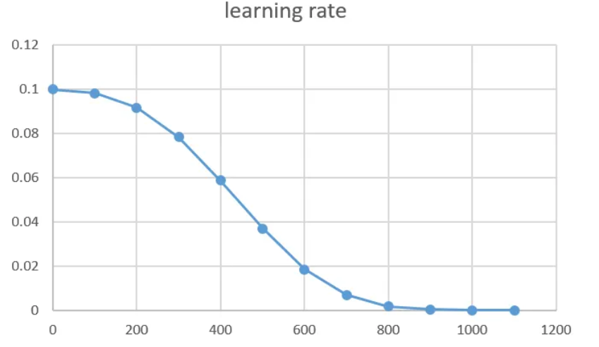
首先,我們設定初始學習率為 0.001,並建立「余弦衰減」調度器(註),
讓學習率隨訓練進程平滑下降,
decay_steps=1000 作為衰減基準,alpha=1e-6(也就是 0.000001),
確保最低學習率不會太小,也避免學習率降得太低而完全停止學習。
接著使用 Adam 優化器搭配這個動態學習率。
損失函數選用 sparse_categorical_crossentropy,跟我們之前使用的不太一樣,
他是專門處理整數標籤的多分類問題,衡量預測與真實答案的差距。
評估指標則包含 accuracy(標準準確率)和 SparseTopKCategoricalAccuracy
(Top-5 準確率,只要正確答案在前 5 個預測中就算對),
後者在實際應用中很有用,比如搜尋引擎只要把正確結果放在前幾名就算成功。
因為我們的標籤是整數形式(如 2 表示第 2 類),
而不是 one-hot 編碼(如 [0,0,1,0,...],我們之前都是用這個),
而Sparse 版本是用來專門處理這種整數標籤格式的好工具,剛好適用於我們現在的實作。
若是還有疑問可以前往我學習時所參考的文章,連結如下:
https://claire-chang.com/2023/01/07/%E4%BA%A4%E5%8F%89%E7%86%B5%E7%9B%B8%E9%97%9C%E6%90%8D%E5%A4%B1%E5%87%BD%E6%95%B8%E7%9A%84%E6%AF%94%E8%BC%83/
這個策略在使用的時候會採用 Cosine 函數,
先使用較大學習率來進行快速收斂,
接著再使用較小學習率收斂,
中間則一定程度規避掉learning rate跨越過大的問題,
也就是說可以讓整體更為「平滑」。
我自己把他理解成:
一開始先快速整個搜索,縮小範圍,
等到縮小(收斂)後再降低速率,類似動態調整的概念。
以上是我們第一階段的內容,明日再戰。

