
昨天看了 linear / GEMM,今天換另一組在 LLM 前向傳播裡常出現的運算子:norm、activation、RoPE。
今天會講三個 torch.ops.sgl_kernel
torch.ops.sgl_kernel.rmsnorm_cpu
torch.ops.sgl_kernel.silu_and_mul_cpu
torch.ops.sgl_kernel.rotary_embedding_cpu
這三類運算子的資料量通常比大 GEMM 小,但它們每一層都會跑,並且常常卡在記憶體存取、reduction、型別轉換和近似函式。它們很適合拿來練習把前面寫過的 RVV 迴圈放進真實運算子。
norm.cpp、activation.cpp、rope.cpp 的 RVV intrinsic 迴圈。先把一個 decoder-only Transformer block 簡化成下面這條路徑:
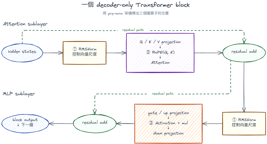
上面的示意圖以 pre-norm 架構為例,綠色虛線是 residual path,①、②、③標出本篇要看的三種運算子。
pre-norm 的 pre 是指 normalization 發生在 Attention 或 MLP 子層之前。以圖中的 Attention 子層為例,輸入 x 會分成兩條路徑:一條先進 RMSNorm 和 Attention,另一條沿 residual path 直接傳到加法節點:
attention_out = x + Attention(RMSNorm(x))
mlp_out       = attention_out + MLP(RMSNorm(attention_out))
這種排法讓 Attention 和 MLP 先接收尺度較一致的輸入,residual path 則保留一條直接傳遞 hidden states 的路徑。相對地,post-norm 會先完成子層運算和 residual add,再做 normalization,例如 LayerNorm(x + Attention(x))。
但不同模型的 norm 擺放方式、activation 種類和 RoPE 設定還是會有差異。
RMSNorm 想要控制 hidden states 的數值尺度。Transformer block 會不斷做線性轉換和 residual add,每個 token 的 hidden vector 大小可能隨層數改變。RMSNorm 在 attention 或 MLP 前先把這個向量調整到可控制的尺度,讓後面的 projection 接收尺度較一致的輸入。
它的功能可以概括成先測量整個向量的 Root Mean Square,再縮放每個 element。對一個 token 的 hidden vector x 來說
rms(x) = sqrt((1 / hidden_size) * Σ x_i² + eps)
out_i  = (x_i / rms(x)) * weight_i
eps 是一個很小的常數,用來避免 rms 太小而造成除法不穩定。weight 則是模型學到的參數,負責再次調整每個 element 的大小。
為了算出 rms,RMSNorm 會先把同一個 token 的所有 element 平方,再把這些平方值加總成一個數值。這種將多個值彙總成一個值的運算就叫 reduction。同一個 token 的所有 element 會共用這個 rms,所以 kernel 要先完成 reduction,才能回頭 normalize 每個 element。
Activation 的目的是讓 MLP 具有非線性的表示能力。連續堆疊 linear layer 仍可以合併成一個線性轉換,中間加入 SiLU 或 GELU 後,模型才能根據輸入產生彎曲的轉換關係。
Activation + mul 的功能還包含 gating,一條分支產生 gate,另一條分支提供要傳遞的值,最後逐元素相乘,調整每個特徵的輸出強度。
以我這裡的 silu_and_mul_cpu 為例,輸入最後一維包含兩組同樣長度的向量。這兩組值通常來自 MLP 的 gate projection 和 up projection
sigmoid(x) = 1 / (1 + exp(-x))
silu(x)    = x * sigmoid(x)
out        = silu(gate) * up
Sigmoid 會產生 0 到 1 之間的平滑係數,SiLU 用它縮放 gate,再和 up 逐元素相乘。從 kernel 角度看,這是連續的 load、exp(-x) 近似、除法和 multiply,沒有 RMSNorm 那種跨整列的 reduction。
RoPE 的目的是把 token 的位置關係放進 attention score。Self-attention 用 Q 和 K 的內積衡量內容關聯,如果沒有額外的位置資訊,這個計算本身就無法分辨 token 在序列中的順序。
RoPE(Rotary Positional Embedding)的功能是依 token position 旋轉 Q/K head 中的成對元素,旋轉發生在 Q/K 內積之前,對一組 (x0, x1) 來說可以寫成:
x0' = x0 * cos(θ) - x1 * sin(θ)
x1' = x1 * cos(θ) + x0 * sin(θ)
高中數甲有學過的旋轉矩陣在這裡出現了,θ 由 position 和這組 hidden dimension 對應的頻率決定。同一個向量在不同 position 會被旋轉不同角度,而旋轉後 Q/K 的內積會包含兩個 token 的相對位置關係。實作時通常預先算好 cos/sin cache,kernel 依 positions 查表,再對 Q 和 K 的 rotary dimension 做逐元素運算。
GEMM 的主要壓力通常來自大矩陣資料搬移和累加器重用,Norm / activation / RoPE 比較像沿著最後一維掃過去。
以 [num_tokens, hidden_size] 的 tensor 來看,這些運算子常見迴圈是:
for each token:
  for hidden dimension:
    load x
    compute
    store out
這種模式很適合 RVV strip-mining:
for (int64_t j = 0; j < hidden_size; j += vl) {
    vl = __riscv_vsetvl_e32m4(hidden_size - j);
    ...
}
但它們也有幾個麻煩的點要去處理,RMSNorm 需要先算整列的 sum of squares,才能做 normalize。只保留 sum 或 scale 這類統計值,第二階段仍要再讀一次 x。想避免從原 tensor 第二次載入,必須保留整列 x;例如與產生 x 的上游運算融合,並讓該列留在可重用的 buffer,和下游運算融合可以省掉 norm output 的 store / reload,但不會消除 RMSNorm 自己的第二次 x 讀取。
Activation 需要近似函式,例如 sigmoid、tanh、erf。RVV intrinsic 沒有直接給完整高階 activation,我在 vector_math.h 有寫一些數學近似函數。
RoPE 要處理 Q/K 的資料配置。有些模型使用 NeoX style,有些使用 interleaved style,兩者的 tensor shape 可以完全一樣,差別在 head dimension 裡哪兩個 element 要組成一個旋轉對。
以 head_dim = 8 的向量 [x0, x1, x2, x3, x4, x5, x6, x7] 為例:
NeoX style:
(x0, x4), (x1, x5), (x2, x6), (x3, x7)

interleaved style:
(x0, x1), (x2, x3), (x4, x5), (x6, x7)
NeoX style 把 head dimension 切成前後兩半,將相同 offset 的 element 配成一組。Interleaved style 則把相鄰的偶數、奇數 index 配成一組。兩種 layout 都套用同一組 cos/sin 旋轉公式,但 kernel 計算配對 index 與載入資料的方式不同。如果 layout 判斷錯誤,程式通常仍能執行,卻會旋轉錯誤的 element,最後影響 attention score。
rmsnorm_cpu 在 sgl-kernel/csrc/cpu/riscv64/norm.cpp
at::Tensor rmsnorm_cpu(at::Tensor& input, at::Tensor& weight, double eps) {
  CHECK_LAST_DIM_CONTIGUOUS_INPUT(input);
  CHECK_INPUT(weight);
  CHECK_DIM(2, input);
  CHECK_DIM(1, weight);
  CHECK_EQ(input.size(1), weight.size(0));
  int64_t batch_size = input.size(0);
  int64_t hidden_size = input.size(1);
  int64_t input_strideN = input.stride(0);
  at::Tensor output = at::empty_like(input);
  ...
  AT_DISPATCH_REDUCED_FLOATING_TYPES(input.scalar_type(), "rmsnorm_kernel", [&] {
    rmsnorm_kernel_impl<scalar_t, false>(
        output.data_ptr<scalar_t>(),
        input.data_ptr<scalar_t>(),
        weight.data_ptr<scalar_t>(),
        batch_size,
        hidden_size,
        input_strideN,
        static_cast<float>(eps));
  });
  return output;
}
這裡先要求 input 最後一維連續,因為 norm 是沿 hidden dimension 掃,如果最後一維不連續,RVV 載入會變麻煩。
RMSNorm 的核心可以拆成兩段
sum = Σ x_i^2
scale = 1 / sqrt(sum / hidden_size + eps)
out_i = x_i * scale * weight_i
第一段 reduction 需要 FP32 累加。BF16 / FP16 input 會先轉成 FP32,再做平方和。下面是 rmsnorm_kernel_impl 的 RVV 主迴圈,我把原本嵌在同一行的 reduction 結果拆成 partial 方便閱讀
float sum_sq = 0.0f;
size_t vl = 0;
vfloat32m1_t vzero = __riscv_vfmv_s_f_f32m1(0.0f, 1);

for (int64_t j = 0; j < hidden_size; j += vl) {
  vl = __riscv_vsetvl_e32m4(hidden_size - j);
  vfloat32m4_t vx = load_as_float_m4(in_ptr + j, vl, scratch);
  vfloat32m4_t vsq = __riscv_vfmul_vv_f32m4(vx, vx, vl);
  vfloat32m1_t partial =
      __riscv_vfredusum_vs_f32m4_f32m1(vsq, vzero, vl);
  sum_sq += __riscv_vfmv_f_s_f32m1_f32(partial);
}
__riscv_vsetvl_e32m4 根據剩餘 element 數設定 vl,同時選擇 FP32(e32)和 LMUL=4(m4)。load_as_float_m4 是我在 vector_helper.h 自己定義的載入函式,會把 BF16 / FP16 輸入轉成 vfloat32m4_t。__riscv_vfmul_vv_f32m4 做 vector-vector 乘法,一次算出 vl 個 x_i²。__riscv_vfredusum_vs_f32m4_f32m1 把 vsq 的 active lanes 加總到 m1 vector 的第一個 lane。__riscv_vfmv_f_s_f32m1_f32 取出該 lane 成為 scalar,再加進 sum_sq。算出整列共用的 rsqrt_var 後,第二趟迴圈會完成 normalize 和 weight 縮放
for (int64_t j = 0; j < hidden_size; j += vl) {
  vl = __riscv_vsetvl_e32m4(hidden_size - j);
  vfloat32m4_t vx = load_as_float_m4(in_ptr + j, vl, scratch);
  vfloat32m4_t vw = load_as_float_m4(weight + j, vl, scratch);
  vfloat32m4_t vnormalized =
      __riscv_vfmul_vf_f32m4(vx, rsqrt_var, vl);
  vfloat32m4_t vout =
      __riscv_vfmul_vv_f32m4(vnormalized, vw, vl);
  store_from_float_m4(out_ptr + j, vout, vl, scratch);
}
vfmul_vf 的 vf 表示 vector 乘 scalar float,適合把同一個 rsqrt_var 套用到所有 lanes;vfmul_vv 再讓每個 lane 乘上各自的 weight。store_from_float_m4 會轉回輸出 dtype 並儲存。最後一段不足一個完整 vector group 時,vsetvl 會縮短 vl 處理尾端。
activation.cpp 裡的 silu_and_mul_cpu 入口是:
at::Tensor silu_and_mul_cpu(const at::Tensor& input) {
  auto input_contig = input.contiguous();
  auto sizes = input.sizes().vec();
  int64_t last_dim = input.ndimension() - 1;
  int64_t d = sizes[last_dim] / 2;
  sizes[last_dim] = d;
  int64_t num_tokens = input.numel() / input.size(-1);
  at::Tensor out = at::empty(sizes, input.options());
  ...
}
它假設最後一維是 2 * d,把前半段當 x,後半段當 y
out = silu(x) * y
這個前置條件必須是最後一維為偶數,目前 C++ 入口直接用整數除法算 d,沒有顯式拒絕 odd size。
如果上層傳入奇數,會遺漏元素並讓後續 token 的 row base 錯位,產生錯誤結果。完整實作應在入口加上偶數檢查,本篇範例只在該條件成立時有效。
每個 token 會呼叫
act_silu_inner(out_ptr + i * d, x_ptr, x_ptr + d, d);
act_silu_inner 的主迴圈有兩路 unroll,這裡先看結構較單純的 tail loop。下方把原本嵌套的表達式拆成暫存變數,觀察 SiLU-and-mul 如何對應到 RVV 運算
size_t vl;
for (; j < d; j += vl) {
  vl = __riscv_vsetvl_e32m4(d - j);
  vfloat32m4_t vx = load_as_float_m4(x_ptr + j, vl, scratch);
  vfloat32m4_t vy = load_as_float_m4(y_ptr + j, vl, scratch);

  vfloat32m4_t vneg_x = __riscv_vfneg_v_f32m4(vx, vl);
  vfloat32m4_t vexp = vfexp_f32m4(vneg_x, vl);
  vfloat32m4_t vdenom = __riscv_vfadd_vf_f32m4(vexp, 1.0f, vl);
  vfloat32m4_t vsigmoid = vrec_f32m4(vdenom, vl);
  vfloat32m4_t vsilu = __riscv_vfmul_vv_f32m4(vx, vsigmoid, vl);
  vfloat32m4_t vout = __riscv_vfmul_vv_f32m4(vsilu, vy, vl);

  store_from_float_m4(out_ptr + j, vout, vl, scratch);
}
這段對應的算式是
vneg_x    = -x
vexp      = exp(-x)
vsigmoid  = 1 / (1 + vexp)
vout      = x * vsigmoid * y
__riscv_vfneg_v_f32m4、__riscv_vfadd_vf_f32m4 和 __riscv_vfmul_vv_f32m4 是 RVV intrinsic。vfexp_f32m4 和 vrec_f32m4 則是我在 vector_math.h 寫的向量數學輔助函式,內部還會繼續用 RVV intrinsic 實作近似運算。像是 vfexp_f32m4 會先做 range reduction,再用 Horner's method 計算多項式:
vfloat32m4_t vz = __riscv_vfmul_vf_f32m4(vx, RVV_LOG2_E, vl);
vint32m4_t vn_int = __riscv_vfcvt_x_f_v_i32m4(vz, vl);
vfloat32m4_t vn = __riscv_vfcvt_f_x_v_f32m4(vn_int, vl);
vfloat32m4_t vf = __riscv_vfsub_vv_f32m4(vz, vn, vl);

vfloat32m4_t vC4 = __riscv_vfmv_v_f_f32m4(RVV_EXP_C4, vl);
vfloat32m4_t vC3 = __riscv_vfmv_v_f_f32m4(RVV_EXP_C3, vl);
vfloat32m4_t poly = __riscv_vfmv_v_f_f32m4(RVV_EXP_C5, vl);
poly = __riscv_vfmadd_vv_f32m4(poly, vf, vC4, vl);
poly = __riscv_vfmadd_vv_f32m4(poly, vf, vC3, vl);
// ...
Horner's method(霍納法)是一種很聰明改寫多項式的方法。例如原本的四次多項式
P(x) = a4*x^4 + a3*x^3 + a2*x^2 + a1*x + a0
可以改寫成
P(x) = (((a4*x + a3)*x + a2)*x + a1)*x + a0
如果每一項都從頭計算 x^k,求值一個 n 次多項式需要 1 + 2 + ... + n 次乘法,時間複雜度是 O(n²)。Horner's method 只需要 n 次乘法與 n 次加法,因此是 O(n)。如果原本已經會重用 x^k,兩者在漸進複雜度上都是 O(n),Horner's method 仍可減少中間暫存值,也不需要先存下多組 x^k。
在 RVV 裡,__riscv_vfmadd_vv_f32m4(poly, vf, coefficient, vl) 剛好可以在一步中計算 poly * vf + coefficient,直接對應 Horner's method 的每一層括號。GELU 路徑則會呼叫 vferf_f32m4 或 vftanh_f32m4,同樣把 erf / tanh 拆成 RVV 可執行的乘加、exp 近似與 reciprocal。
這種運算子的效能常常受到兩件事影響。
1.近似函式本身的指令量,SiLU 需要 sigmoid,GELU 需要 tanh 或 erf,指令比單純 multiply 多。
2.input/output 頻寬,每個元素通常載入兩份 input,儲存一份 output。如果 hidden size 大,記憶體流量仍然可觀。
rotary_embedding_cpu 在 rope.cpp。入口會先檢查形狀
TORCH_CHECK(
    input_dim == 2 || input_dim == 3 || input_dim == 4,
    " Query/Key must be 2D ... or 3D ... or 4D ... tensor");
CHECK_LAST_DIM_CONTIGUOUS_INPUT(query);
CHECK_LAST_DIM_CONTIGUOUS_INPUT(key);
它支援 2D、3D、4D input
2D: [num_tokens, num_heads * head_size]
3D: [num_tokens, num_heads, head_size]
4D: [batch_size, seq_len, num_heads, head_size]
這三種 shape 表達的 Q/K 內容相似,主要差在 token、batch 和 head 維度是否被展平,以及目前 RVV kernel 為各路徑提供的功能
| Shape | 資料如何排列 | 目前 RVV 路徑 |
|---|---|---|
| 2D | 每列是一個 token,所有 heads 展平放在最後一維;kernel 用 head_size 推回 head 數量 |
支援 NeoX 與 interleaved,Q/K 可有不同 head 數,並直接在原本 Q/K 上修改(in-place) |
| 3D | token 仍是第一維,head 被拆成獨立維度,沒有單獨的 batch 維度 | 目前只支援 interleaved、要求 K 只有 1 個 head,並另外建立輸出 tensor(out-of-place) |
| 4D | 完整保留 batch、sequence 和 head 三個維度,batch_size * seq_len 要和 positions 的元素數一致 |
支援 NeoX 與 interleaved,Q/K 可有不同 head 數,並原地修改 Q/K |
例如同樣是 32 個 heads、head_size = 128,2D 會把一個 token 存成長度 4096 的一列;3D/4D 則保留 [32, 128] 這兩個維度。RoPE 使用的旋轉公式沒有變,kernel 需要依 shape 算出每個 token 和 head 的起始位置。
RoPE 會根據 positions 去 cos_sin_cache 找對應 cos/sin,然後對 Q/K 的 rotary dimension 做旋轉。
簡化公式可以寫成
x0' = x0 * cos - x1 * sin
x1' = x1 * cos + x0 * sin
麻煩在資料配置,NeoX style 和 interleaved style 的配對方式不同,kernel 需要知道哪兩個元素是一組,才能正確旋轉。
先看 interleaved style 的 RVV 主迴圈。因為要配對 (x0, x1)、(x2, x3),kernel 用 stride-2 load 分別取出偶數與奇數 index:
const ptrdiff_t stride = 2 * static_cast<ptrdiff_t>(sizeof(scalar_t));
size_t vl = 0;

for (int64_t j = 0; j < embed_dim; j += vl) {
  vl = __riscv_vsetvl_e32m4(embed_dim - j);
  vfloat32m4_t v_cos = load_as_float_m4(cos_ptr + j, vl, scratch);
  vfloat32m4_t v_sin = load_as_float_m4(sin_ptr + j, vl, scratch);
  vfloat32m4_t v_x =
      load_strided_as_float_m4(head_ptr + 2 * j, stride, vl, scratch);
  vfloat32m4_t v_y =
      load_strided_as_float_m4(head_ptr + 2 * j + 1, stride, vl, scratch);

  vfloat32m4_t v_out_x = __riscv_vfmul_vv_f32m4(v_x, v_cos, vl);
  v_out_x = __riscv_vfnmsac_vv_f32m4(v_out_x, v_y, v_sin, vl);
  vfloat32m4_t v_out_y = __riscv_vfmul_vv_f32m4(v_y, v_cos, vl);
  v_out_y = __riscv_vfmacc_vv_f32m4(v_out_y, v_x, v_sin, vl);

  store_strided_from_float_m4(head_ptr + 2 * j, stride, v_out_x, vl, scratch);
  store_strided_from_float_m4(head_ptr + 2 * j + 1, stride, v_out_y, vl, scratch);
}
這裡有兩個和公式直接對應的 fused multiply-accumulate intrinsic
vfnmsac(v_out_x, v_y, v_sin) 計算 v_out_x - v_y * v_sin,完成 x * cos - y * sin。vfmacc(v_out_y, v_x, v_sin) 計算 v_out_y + v_x * v_sin,完成 y * cos + x * sin。NeoX style 的乘加 intrinsic 相同,載入方式不同。它要配對前後半,所以用 x_index = j 和 y_index = embed_dim + j,再用連續的 load_as_float_m4 載入兩段資料。這也是 layout 會直接改變 RVV memory access 的地方。
RVV 寫 RoPE 時,要注意幾件事
這些檢查看起來瑣碎,但對推論服務很重要,資料配置錯了不一定 crash,可能只是模型輸出錯。
呼叫端需要依照實際 shape 處理各路徑的前置條件與輸出語意,特別是 3D 路徑的單一 KV head 限制與 out-of-place 輸出。
K1 的 Vector-256bit 對這些運算子的影響比較直觀
Benchmark 時可以看幾個訊號
sgl-kernel::rmsnorm_cpu、sgl-kernel::silu_and_mul_cpu、sgl-kernel::rotary_embedding_cpu。今天看了 linear 以外的三類 RVV 運算子
明天會講 attention kernel, attention 會把今天的 reduction、activation-like softmax、資料配置、KV cache、GEMM-like dot product 放在同一個 kernel 裡。
sgl-kernel/csrc/cpu/riscv64/norm.cppsgl-kernel/csrc/cpu/riscv64/activation.cppsgl-kernel/csrc/cpu/riscv64/rope.cpp



 iThome鐵人賽
 看影片追技術