從宏觀走向區域維度

確認完月營收大盤後，下一個關鍵問題是：「營收來自哪裡？消費者的購買習慣有區域差異嗎？」

今天我們以昨天篩選出的有效訂單 valid_orders 為基礎，將視角下鑽至地理維度，
計算各州的訂單集中度與平均客單價（Average Order Value, AOV），並用圖表直觀呈現洞察。

步驟一：依州別聚合關鍵指標

使用 groupby 針對買家所在州別（customer_state）進行聚合，同時計算單量、營收與客單價：

# 依客戶州別分組，計算單量與營收
state_summary = valid_orders.groupby('customer_state').agg(
    order_count=('order_id', 'count'),
    total_gmv=('total_item_price', 'sum')
).reset_index()

# 計算客單價 (AOV) 與單量佔比 (%)
state_summary['aov'] = (state_summary['total_gmv'] / state_summary['order_count']).round(2)
state_summary['order_share_pct'] = (state_summary['order_count'] / state_summary['order_count'].sum() * 100).round(2)

步驟二：單量集中度 vs. 客單價反差

透過兩種不同排序，能立刻看出明顯的商業反差：

# 1. 依單量排序（看市場規模）
state_summary.sort_values(by='order_count', ascending=False).head(5)

# 2. 依客單價排序（看消費單價）
state_summary.sort_values(by='aov', ascending=False).head(5)

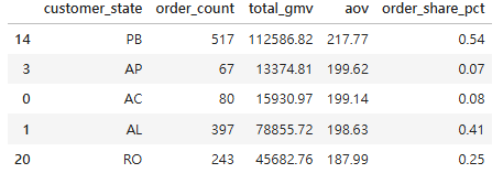
高客單榜首（PB 帕拉伊巴州）：
客單價高達 217.77 BRL，是全平台客單價最高的州，平均每筆訂單消費力最驚人。

高單價群聚（AP、AC、AL、RO）：
其餘入榜州別的客單價也全面落在 188～200 BRL 的高檔區間（AP 199.62、AC 199.14、AL 198.63、RO 187.99）。

極端反差（單量極低）：
這 5 個高客單州的單量佔比（order_share_pct）全部低於 0.6%（AP 和 AC 甚至只有 0.07% 與 0.08%），五州合計單量佔比不到 1.4%。

實作區 :

步驟三：用雙圖直擊核心論點

在資料清洗完備的前提下，繪製圖表時保持「一張圖講清楚一個結論」：

import matplotlib.pyplot as plt
import seaborn as sns

plt.style.use('seaborn-v0_8-whitegrid')
fig, (ax1, ax2) = plt.subplots(1, 2, figsize=(14, 5))

# 圖一：單量 Top 10 州別（集中度）
top_vol = state_summary.sort_values(by='order_count', ascending=False).head(10)
sns.barplot(data=top_vol, x='customer_state', y='order_count', ax=ax1, palette='Blues_r')
ax1.set_title('Top 10 States by Order Volume', fontsize=12, fontweight='bold')
ax1.set_xlabel('State')
ax1.set_ylabel('Order Count')

# 圖二：客單價 Top 10 州別（高單價市場）
top_aov = state_summary.sort_values(by='aov', ascending=False).head(10)
sns.barplot(data=top_aov, x='customer_state', y='aov', ax=ax2, palette='Reds_r')
ax2.set_title('Top 10 States by AOV (BRL)', fontsize=12, fontweight='bold')
ax2.set_xlabel('State')
ax2.set_ylabel('AOV (BRL)')

plt.tight_layout()
plt.show()

實作區 :　

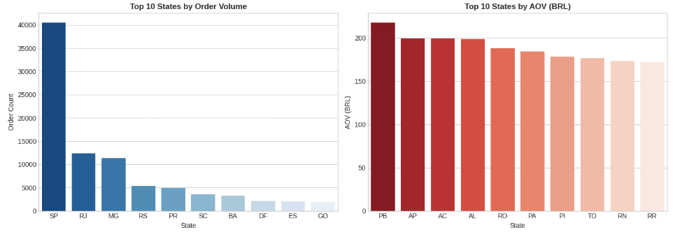
1.掌握 80/20 法則： 平台訂單高度依賴東南部大州，供應鏈重心明確。

2.釐清客單價反差： 核心市場重頻次與單量，偏遠市場重高客單耐久財。

3.完成首張商業圖表： 以雙指標長條圖呈現市場結構。

偏遠地區消費者願意支付高客單價，但他們承擔了多少運費？物流天數是否過長？
明天我們將切入電商最關鍵的履約成本，展開運費比率與配送延遲分析！