目前至今可以得到以一個多項式來描述車道線,提供有門檻值圖像,估計哪些像素屬於左右車道線(如下圖以紅色和藍色顯示),接著,我們將計算符合車道線之曲率半徑。
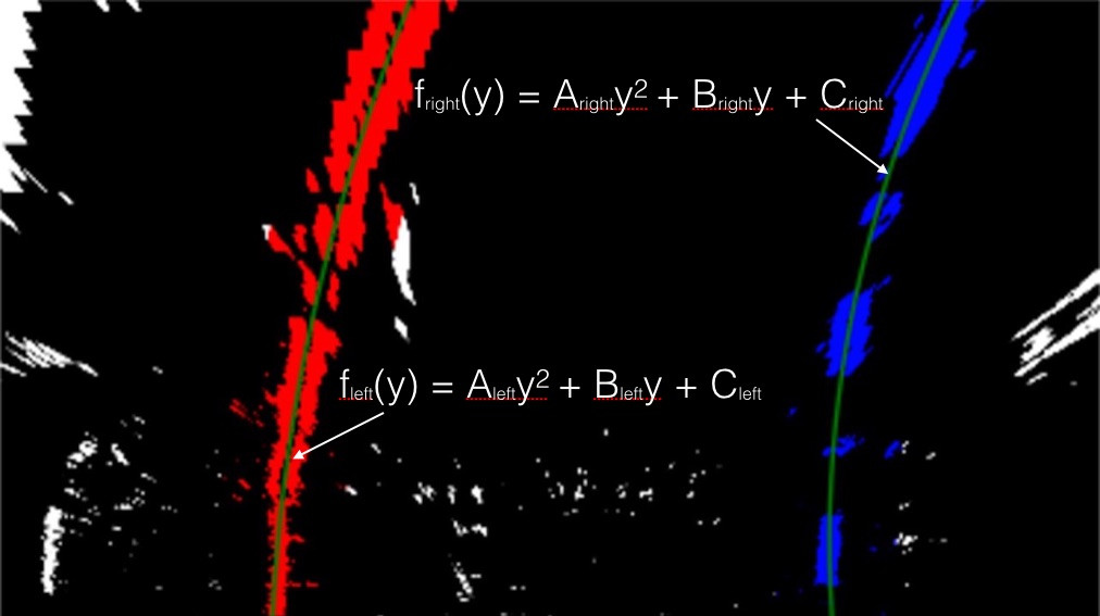
我們用以下二元多項式來描述車道線:
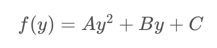
在此主要係描述f(y),而非f(x),由於包裝後圖像中的車道線接近垂直,並且對於多個y值可能具有相同的x值。
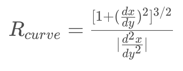
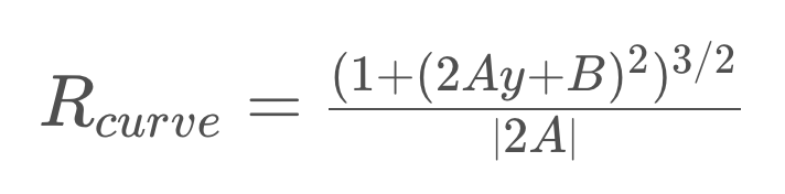
針對任何點X,給定曲率半徑,x=f(y)如下:
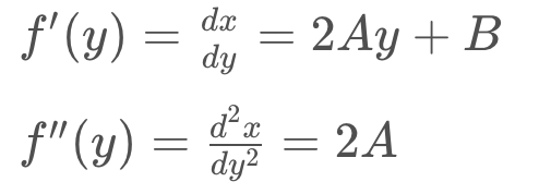
在上述二階多項式的情況下,一階和二階導數是:
因此,我們的曲率半徑方程式為:
import numpy as np
import matplotlib.pyplot as plt
# Generate some fake data to represent lane-line pixels
ploty = np.linspace(0, 719, num=720)# to cover same y-range as image
quadratic_coeff = 3e-4 # arbitrary quadratic coefficient
# For each y position generate random x position within +/-50 pix
# of the line base position in each case (x=200 for left, and x=900 for right)
leftx = np.array([200 + (y**2)*quadratic_coeff + np.random.randint(-50, high=51)
                              for y in ploty])
rightx = np.array([900 + (y**2)*quadratic_coeff + np.random.randint(-50, high=51)
                                for y in ploty])

leftx = leftx[::-1]  # Reverse to match top-to-bottom in y
rightx = rightx[::-1]  # Reverse to match top-to-bottom in y


# Fit a second order polynomial to pixel positions in each fake lane line
left_fit = np.polyfit(ploty, leftx, 2)
left_fitx = left_fit[0]*ploty**2 + left_fit[1]*ploty + left_fit[2]
right_fit = np.polyfit(ploty, rightx, 2)
right_fitx = right_fit[0]*ploty**2 + right_fit[1]*ploty + right_fit[2]

# Plot up the fake data
mark_size = 3
plt.plot(leftx, ploty, 'o', color='red', markersize=mark_size)
plt.plot(rightx, ploty, 'o', color='blue', markersize=mark_size)
plt.xlim(0, 1280)
plt.ylim(0, 720)
plt.plot(left_fitx, ploty, color='green', linewidth=3)
plt.plot(right_fitx, ploty, color='green', linewidth=3)
plt.gca().invert_yaxis() # to visualize as we do the images
輸出如下: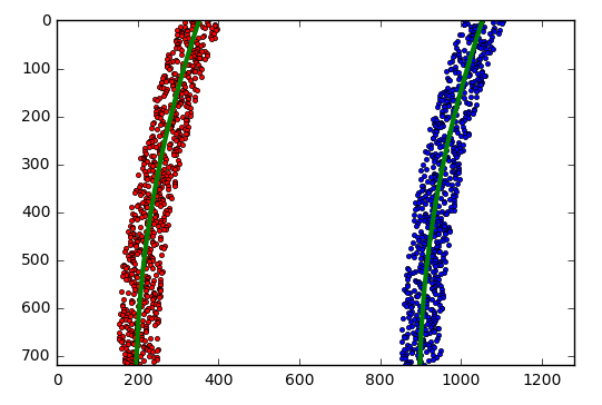


 iThome鐵人賽