昨天學習了一些基本概念
今天要來看python 實作

今天的sample data

在線性回歸之前

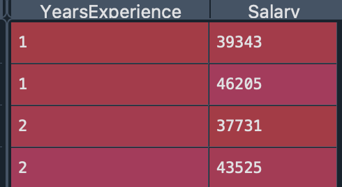
再進入線性回歸之前, 我們需要對資料做前處理
這裡用的是之前範本裡的code

1. 載入 Salary_Data.csv (今天的資料集）
2. 設定自變量x與應變量y, x是Experience 欄位的所有資料, y是Salary欄位的所有資料
3. 將資料的2/3 歸為training set, 1/3歸為testing set
   training set 包含 x_train, y_train, 會將這些數據拿來train model
   testing set 包含 x_test, y_test, 用來驗證train 完成的model的準確性
4. 這邊我們不用做feature scaling(特徵縮放)因為今天會用到的python library 預設會幫我們做好
   (大部分的library 都會內建feature scaling)

dataset = pd.read_csv('Salary_Data.csv')
x = dataset.iloc[:, :-1].values
y = dataset.iloc[:, 1].values
x_train, x_test, y_train, y_test = train_test_split(x,y,test_size=1/3, random_state=0)

進入正題 simple linear regression in python

我們使用的是sklearn.linear_model 裡的 LinearRegression class

1. 創建一個LinearRregression 物件叫regressor
2. 呼叫fit() 帶入training set 資料進行擬合, 代表這行程式碼結束後model 就被訓練好了
3. 呼叫predict()帶入x_train 資料來測試model的結果, 將結果存入y_pred

from sklearn.linear_model import LinearRegression
regressor = LinearRegression()
regressor.fit(x_train, y_train)
y_pred = regressor.predict(x_test)

是時候驗收成果了
這時候可以用Vairable Explorer 看到 y_pred 和 y_test 的資料
看看機器預測的結果跟實際結果差多少
可以發現大部分預測都還算成功, 但仍有資料(ex: 第七筆）有誤差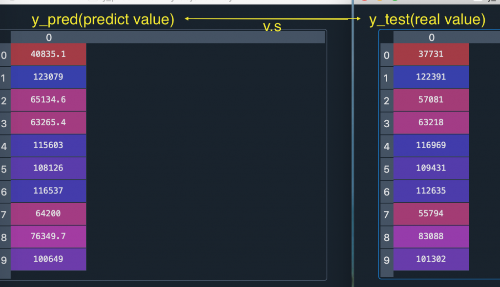

用python 畫圖

只看數據沒有感覺, 我們可以把model 最重要的線給畫出來
這裡會畫兩張圖, 不過方法都是一樣的, 我以第一張圖來說明function

1. 呼叫scatter() 帶入 training data 畫出training data 中的每一個點, 並指定用紅色
2. 呼叫plot()帶入x_train 和用x_train套入模型得到的y軸預測值畫出直線, 並指定用藍色
3. 呼叫title()設定圖表名稱
4. 呼叫xlabel(), ylabel()設定x, y 軸名稱
5. 呼叫show() 畫出圖型

第二張圖預計呈現的是 testing data 和 model 的差異
因此散點帶入testing data(當作答案）
直線則用 x_train 和 regressor predict 出的y值來畫

注意：第二張圖的plot()跟第一張帶一樣的參數, 原因是
regressor 是套用x_train 跟 y_train 來訓練model
因此不管是用predict(x_train) or predict(x_test) 都會得到一樣的線
因為背後都是同一個regressor

import matplotlib.pyplot as plt
plt.scatter(x_train, y_train, color = 'red')
plt.plot(x_train, regressor.predict(x_train), color = 'blue')
plt.title("Salary v.s Experience (training set)")
plt.xlabel('Years of Experience')
plt.ylabel('Salary')
plt.show()

plt.scatter(x_test, y_test, color = 'red')
plt.plot(x_train, regressor.predict(x_train), color = 'blue')
plt.title("Salary v.s Experience (testing set)")
plt.xlabel('Years of Experience')
plt.ylabel('Salary')
plt.show()

第一張表達的是training data set 和 model 的關係
可以看到大部分的資料跟model 都很接近, 不過仍然有一些點有誤差

第二張圖是testing data set 和model 的關係
紅色點的y軸是機器預測值, 跟model 也相當接近

完整程式碼

# -*- coding: utf-8 -*-
"""
Editor: Ironcat45
Date: 2022/09/23
"""

import numpy as np
import pandas as pd
from sklearn.model_selection import train_test_split

"""
1. <Data preprocessing>
   1. load the Salary_Data.csv
   2. read the "experience" column as x
      read the "salary" column as y
   3. split the data to the trainset(2/3) and testset(1/3)
"""
dataset = pd.read_csv('Salary_Data.csv')
x = dataset.iloc[:, :-1].values
y = dataset.iloc[:, 1].values
x_train, x_test, y_train, y_test = train_test_split(x,y,test_size=1/3, random_state=0)

"""
2. <Linear regression>
   Fitting simple linear regression to the training set
   1. create an LinearRegression obj named regressor
   2. fit the x_train and y_train data(so now the regression is done)
   3. note that we don't have to deal with feature scaling since
      the class LinearRegression contains this step automatically
"""
from sklearn.linear_model import LinearRegression
regressor = LinearRegression()
regressor.fit(x_train, y_train)

"""
3. <Linear regression>
   Predicting the test set results
"""
y_pred = regressor.predict(x_test)

"""
4. Visualising the training set results
"""
import matplotlib.pyplot as plt
plt.scatter(x_train, y_train, color = 'red')
plt.plot(x_train, regressor.predict(x_train), color = 'blue')
plt.title("Salary v.s Experience (training set)")
plt.xlabel('Years of Experience')
plt.ylabel('Salary')
plt.show()

plt.scatter(x_test, y_test, color = 'red')
plt.plot(x_train, regressor.predict(x_train), color = 'blue')
plt.title("Salary v.s Experience (testing set)")
plt.xlabel('Years of Experience')
plt.ylabel('Salary')
plt.show()