昨天介紹了Pix2Pix的原理,Pix2Pix可以達成許多影像處理的任務,其中的U-Net也是目前較常用的架構。今天就來看看Pix2Pix模型要如何建立起來,今天的模型複雜度會比之前介紹的要更複雜一點,若有不理解的請不吝發問,我會盡力解答!
今天要建立Pix2Pix模型,快速複習一下Pix2Pix的特點,想了解更多歡迎參考我昨天的文章:
今天要帶各位實作的是使用Pix2Pix來做mnist手寫資料的圖像修復。圖像修復顧名思義就是使用被毀損的圖片 (或將圖像一部分毀損),將毀損圖片作為條件輸入至網路中,訓練模型將圖片還原。
函式庫的匯入與前幾天差不多,但為了更了解模型架構,所以使用了plot_model方法。
plot_model這個方法必須pip install pydot與安裝graphviz,後者需要到網路上下載並設定環境變數,詳情可以看看其他教學。
另外使用了跳接 (Skip Connect),所以會使用Keras的Concatenate來連接不同網路層的輸出;以及使用損失函數的部分,”binary_crossentropy”與”mae”這部分也可在編譯模型時直接用字串來指定,不過這次就匯入給各位看,各位也可以看看其他損失函數的使用。完整函式庫匯入如下。
from tensorflow.keras.datasets import mnist
from tensorflow.keras.layers import Input, BatchNormalization, LeakyReLU, Activation, Conv2DTranspose, Conv2D, Concatenate, Dropout
from tensorflow.keras.models import Model, save_model
from tensorflow.keras.optimizers import Adam
import matplotlib.pyplot as plt
import numpy as np
import os
from tensorflow.keras.utils import plot_model
from tensorflow.keras.losses import BinaryCrossentropy, MeanAbsoluteError #匯入損失函數
這一步的資料前處理我們要手動將圖部份給遮蓋住,那遮蓋面積與遮蓋區域是完全隨機的。最終遮蓋的效果會如下:
那來看看程式碼如何實現吧:
前面都一樣,從mnist匯入資料,接著我們取前10000筆資料做訓練,這部分主要是因為使用60000筆然後為每筆資料都遮蓋會花比較久的時間,所以為了節省時間先取10000筆。
接著處理資料,正規化等。然後就是要建立對應的毀損資料了,我們使用Numpy的copy功能複製陣列並賦值給destroy_x_train,像這樣:destroy_x_train = x_train.copy()。
接著建立遮蓋區域,首先先隨機挑選出遮蓋的左上角,以及隨機指定寬度,然後就可以建立遮蓋區域了,如下圖: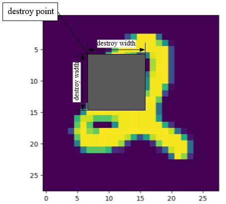
接著就是將每一張照片進行遮蓋,遮蓋就是把那個部份的像素改成一個數字就好了,我是使用0,在反轉換回來時會變成0.5所以就變成灰色了。接著就是刪除不必要的變數,這部分也非必要,但為了節省記憶體空間還是可以刪一下~最後self.show_processed_image(img=x_train, processed_img=destroy_x_train)方法是提供給我們預覽處理過後圖片的樣子。
def load_data(self):
        (x_train, _), (_, _) = mnist.load_data()
        x_train = x_train[:10000,:,:] #處理60000張照片比較久,故使用10000張照片就好
        x_train = (x_train / 127.5)-1
        x_train = x_train.reshape((-1, 28, 28, 1))
        destroy_x_train = x_train.copy() #要準備毀損的照片
        destroy_point = np.random.randint(low=3, high=15, size=(10000, )) #遮蔽地點的最左上角
        destroy_width = np.random.randint(low=8, high=13, size=(10000, )) #遮蔽面的寬度
        destroy_area = destroy_point+destroy_width #遮蔽地點的右下角
        #將每一張圖片根據其左上角到右下角建立一個灰色正方形的遮蔽部分
        for i in range(10000):
            #print進度
            print(f'\rDestroying the images... finish:{round(i/100,3)}%', end='')
            destroy_x_train[i, destroy_point[i]:destroy_area[i], destroy_point[i]:destroy_area[i], 0] = 0

        del destroy_point, destroy_width, destroy_area #刪除用不到的變數,節省記憶體空間
        # self.show_processed_image(img=x_train, processed_img=destroy_x_train)
        return x_train, destroy_x_train
show_processed_image方法定義如下,就是一些Matplotlib排版的東東,與顯示圖片的部分而已。
def show_processed_image(self, img, processed_img):
        l_x_train = (processed_img + 1) / 2
        x_train = (img + 1) / 2
        fig, axs = plt.subplots(4, 4)
        count = 0
        axs[0, 0].set_title('Masked Image')
        axs[0, 1].set_title('Origin Image')
        axs[0, 2].set_title('Masked Image')
        axs[0, 3].set_title('Origin Image')
        for i in range(4):
            axs[i, 0].imshow(l_x_train[count, :, :, 0], cmap='gray')  # 毀損圖片
            axs[i, 0].axis('off')
            axs[i, 1].imshow(x_train[count, :, :, 0], cmap='gray')  # 生成圖片
            axs[i, 1].axis('off')
            axs[i, 2].imshow(l_x_train[count + 4, :, :, 0], cmap='gray')  # 毀損圖片
            axs[i, 2].axis('off')
            axs[i, 3].imshow(x_train[count + 4, :, :, 0], cmap='gray')  # 生成圖片
            axs[i, 3].axis('off')
            count += 1
        plt.show()
接著就是建立Pix2Pix類別了。需要注意的是patchGAN的shape大小,昨天有提,Pix2Pix的判別器會將圖片切成很多小圖片,接著再判斷這些小圖片的真假,所以我們要定義一個這些部份的shape,之後的真假標籤就是依據這些大小判斷。麻煩的是這部分的shape通常會用手算出來,或者直接使用model.summary()來確認輸出的shape!
class Pix2Pix():
    def __init__(self, generator_lr, discriminator_lr):
        if not os.path.exists('./result/Pix2Pix/imgs'):
            os.makedirs('./result/Pix2Pix/imgs')

        self.generator_lr = generator_lr
        self.discriminator_lr = discriminator_lr
        #建立損失
        self.cross_entropy = BinaryCrossentropy(from_logits=True)
        self.l1 = MeanAbsoluteError()

        self.discriminator = self.build_discriminator()
        self.generator = self.build_generator()
        self.adversarial = self.build_adversarialmodel()
        #建立patcgGAN要判斷的圖片大小
        self.discriminator_patch = (7, 7, 1)
        self.gloss = []
        self.dloss = []
定義模型的部分也有許多東西要注意,這邊再提醒一次重點:
生成器:因為mnist的圖片只是(28, 28, 1)的shape,並不是解析度高的彩色圖,所以這裡的U-Net就簡單設計就好~另外U-Net的跳接務必確認shape有沒有對上,否則張量合併時會出現錯誤。
CNN的shape設計有一些重點,以下假設輸入shape是(28, 28, 1)的話:
unit為n,strides為m的Conv2D後輸出形狀會變成(28/m, 28/m, n)unit為n,strides為m的Conv2DTranspose後輸出形狀會變成(28*m, 28*m, n)padding='same'的情況下,padding=’valid’則需要再考慮卷積核大小的影響。第一層與最後一層都不使用批次正規化 (BN)。
def build_generator(self):
        def UpSampling(input_, unit, kernel_size, strides=2, bn=True):
            #上採樣層使用ReLU
            x = Conv2DTranspose(unit, kernel_size=kernel_size, strides=strides, padding='same')(input_)
            x = Activation('relu')(x)
            if bn:
                x = BatchNormalization(momentum=0.8)(x)
            return x
        def DownSampling(input_, unit, kernel_size, strides=2, bn=True):
            #下採樣層使用LeakyReLU
            x = Conv2D(unit, kernel_size=kernel_size, strides=strides, padding='same')(input_)
            x = LeakyReLU(alpha=0.2)(x)
            if bn:
                x = BatchNormalization(momentum=0.8)(x)
            return x

        input_ = Input(shape=(28, 28, 1))
        #建立一個淺層的U-Net,要注意shape有沒有對上,這部分需要手動計算
        d1 = DownSampling(input_, unit=32, kernel_size=4, bn=False) #shape=(14,14,32)
        d2 = DownSampling(d1, unit=64, kernel_size=4) #shape=(7,7,64)
        latent = DownSampling(d2, unit=128, kernel_size=4, strides=1) #shape=(7,7,128)
        u1 = UpSampling(latent, unit=64, kernel_size=4, strides=1) #shape=(7,7,64)
        u1 = Concatenate(axis=-1)([u1, d2])
        u2 = UpSampling(u1, unit=32, kernel_size=4) #shape=(14,14,32)
        u2 = Concatenate(axis=-1)([u2, d1])
        out = Conv2DTranspose(1, kernel_size=4, strides=2, padding='same', activation='tanh')(u2)

        model = Model(inputs=input_, outputs=out, name='Generator')
        model.summary()
        plot_model(model=model,to_file='./result/Pix2Pix/Generator.png',show_shapes=True)
        return model
我們使用兩層下採樣層,一層隱向量層,兩層上採樣層包含跳接,最後的模型圖如下圖 (使用plot_model生成,然後show_shapes=True代表顯示每層的輸出shape):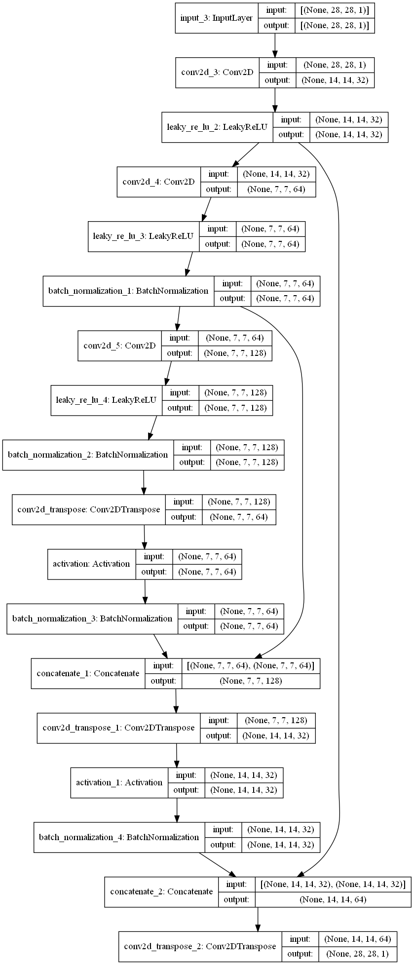
判別器:判別器則須注意PatchGAN架構,以及要判斷這張圖片是不是有遵循條件 (被遮擋的圖片)生成,所以要建立兩個輸入。
接著習慣上來說,看生成器有幾個下採樣層,判別器就使用幾個下採樣層。
最後再建立輸出層。注意第一層與最後一層都不使用批次正規化 (BN)。
def build_discriminator(self):
        def DownSampling(input_, unit, kernel_size, strides=2, bn=True):
            x = Conv2D(unit, kernel_size=kernel_size, strides=strides, padding='same')(input_)
            x = LeakyReLU(alpha=0.2)(x)
            if bn:
                x = BatchNormalization(momentum=0.8)(x)
            x = Dropout(0.3)(x)
            return x
        image_input = Input(shape=(28, 28, 1))
        destory_image_input = Input(shape=(28, 28, 1))
        input_ = Concatenate(axis=-1)([image_input, destory_image_input])

        x = DownSampling(input_, unit=32, kernel_size=4, bn=False)
        x = DownSampling(x, unit=64, kernel_size=4)
        out = Conv2D(1, kernel_size=4, strides=1, padding='same')(x)

        model = Model(inputs=[image_input, destory_image_input], outputs=out, name='Discriminator')
        dis_optimizer = Adam(learning_rate=self.discriminator_lr , beta_1=0.5)
        model.compile(loss=self.cross_entropy,
                      optimizer=dis_optimizer,
                      metrics=['accuracy'])
        model.summary()
        plot_model(model=model, to_file='./result/Pix2Pix/Discriminator.png', show_shapes=True)
        return model
模型的最終結果如下: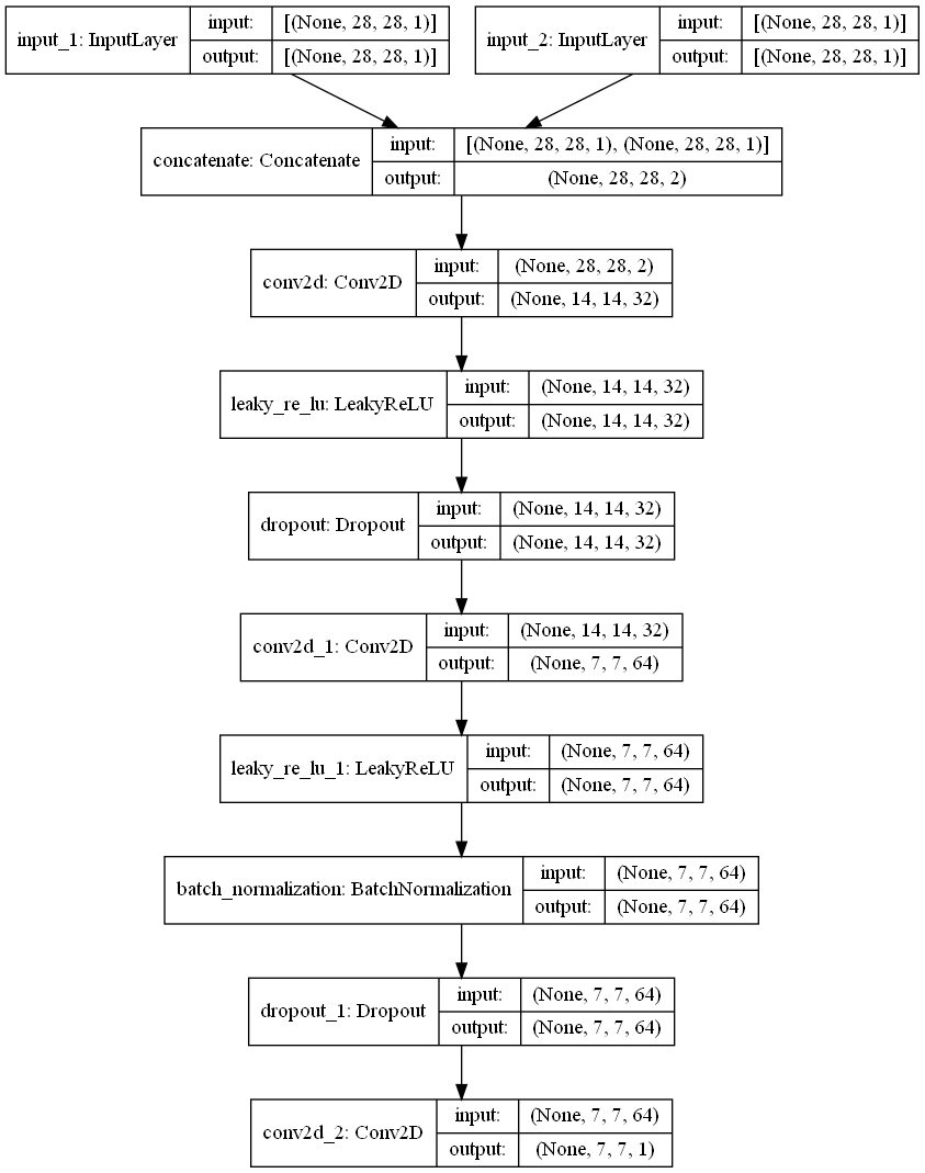
可以看到輸出的shape是 (None, 7, 7, 1),None代表批次量,這部分在訓練model時會自動計算。
對抗模型:對抗模型也有一些細節要注意的,可以對照下面標號與程式碼部分來理解:
loss_weights=[1, 100]。代表總損失是交叉熵+100*L1損失。程式碼如下:
def build_adversarialmodel(self):
        #1.
        destory_image_input = Input(shape=(28, 28, 1))
        #2.
        generator_sample = self.generator(destory_image_input)
        #3
        self.discriminator.trainable = False
        out = self.discriminator([generator_sample, destory_image_input])
        #4
        model = Model(inputs=destory_image_input, outputs=[out, generator_sample])
        #5
        adv_optimizer = Adam(learning_rate=self.generator_lr, beta_1=0.5)
        model.compile(loss=[self.cross_entropy, self.l1], loss_weights=[1, 100], optimizer=adv_optimizer)
        plot_model(model=model, to_file='./result/Pix2Pix/Adversarial.png', show_shapes=True)
        model.summary()
        return model
另外以上的模型可以依據個人喜好設計,只要掌握以上原則,建立出合理的模型就好。如果訓練效果不佳可能是損失函數設定的不好,或者模型架構有問題,太淺或太深,要再慢慢修正。
訓練步驟:
訓練步驟也要注意一下根據模型建立時的輸入部分,輸入別搞錯了喔。
以及判別器PatchGAN的標籤也要定義好,要注意shape不要搞錯了。
還有對抗模型在訓練時要與真實圖片與真實標籤去計算誤差,之前曾經不小心把生成圖片丟進去,導致訓練出一坨答辯,需要引以為戒。
生成器訓練的損失有三個,第一個是損失加總、第二個是交叉熵 (未經過加權)、第三個是L1損失 (未經過加權)。
def train(self, epochs, batch_size=128, sample_interval=50):
        # 準備訓練資料
        x_train, destroy_x_train = self.load_data()
        #標籤要對照上使用PatchGAN的shape
        valid = np.ones((batch_size, ) + self.discriminator_patch)
        fake = np.zeros((batch_size, ) + self.discriminator_patch)
        for epoch in range(epochs):
            idx = np.random.randint(0, x_train.shape[0], batch_size)
            imgs = x_train[idx]
            destory_img = destroy_x_train[idx]
            gen_imgs = self.generator.predict(destory_img)
            #輸入別搞混了,別把遮擋圖與原圖給輸入相反了
            d_loss_real = self.discriminator.train_on_batch([imgs, destory_img], valid)
            d_loss_fake = self.discriminator.train_on_batch([gen_imgs, destory_img], fake)
            d_loss = 0.5 * np.add(d_loss_real, d_loss_fake)
            self.dloss.append(d_loss[0])
            #對抗模型訓練時要注意是要與真實標籤與真實圖去計算誤差
            g_loss = self.adversarial.train_on_batch(destory_img, [valid, imgs])
            self.gloss.append(g_loss)
            print(f"Epoch:{epoch} [D loss: {d_loss[0]:.4f}, acc: {100 * d_loss[1]:.2f}] [G loss: Total:{g_loss[0]:.4f}, crossentropy loss:{g_loss[1]:.4f}, L1 loss:{g_loss[2]:.6f}]")
            if epoch % sample_interval == 0:
                self.sample(epoch)
        self.save_data()
儲存資料的部分都沒有變:
def save_data(self):
        np.save(file='./result/Pix2Pix/generator_loss.npy',arr=np.array(self.gloss))
        np.save(file='./result/Pix2Pix/discriminator_loss.npy', arr=np.array(self.dloss))
        save_model(model=self.generator,filepath='./result/Pix2Pix/Generator.h5')
        save_model(model=self.discriminator,filepath='./result/Pix2Pix/Discriminator.h5')
        save_model(model=self.adversarial,filepath='./result/Pix2Pix/Adversarial.h5')
圖片的顯示也是有稍微排過,一次顯失毀損圖、生成圖、真實圖,這樣比較好對比訓練過程:
def sample(self, epoch=None, num_images=9, save=True):
        r = int(np.sqrt(num_images))
        idx = [100, 200, 300] #手動隨機挑三張照片,比較好觀察變化
        x_train, destroy_x_train = self.load_data()
        destory_img = destroy_x_train[idx]
        x_train = x_train[idx]
        gen_imgs = self.generator.predict(destory_img)
        gen_imgs = (gen_imgs+1)/2
        fig, axs = plt.subplots(r, r)
        count = 0
        axs[0, 0].set_title('Destory image')
        axs[0, 1].set_title('Generative image')
        axs[0, 2].set_title('Real image')
        for i in range(r):
            axs[i, 0].imshow(destory_img[count, :, :, 0], cmap='gray')  #毀損圖片
            axs[i, 0].axis('off')
            axs[i, 1].imshow(gen_imgs[count, :, :, 0], cmap='gray') #生成圖片
            axs[i, 1].axis('off')
            axs[i, 2].imshow(x_train[count, :, :, 0], cmap='gray')  #真實圖片
            axs[i, 2].axis('off')
            count += 1
        if save:
            fig.savefig(f"./result/Pix2Pix/imgs/{epoch}epochs.png")
        else:
            plt.show()
        plt.close()
然後就可以訓練了,訓練了幾次後發現mnist大約10000次以內就可以訓練好,不過再更複雜一點的資料集可能就需要更多訓練次數了。
| 參數 | 參數值 |
|---|---|
| 生成器學習率 | 0.0002 |
| 判別器學習率 | 0.0002 |
| Batch Size | 64 |
| 訓練次數 | 10000 |
if __name__ == '__main__':
    gan = Pix2Pix(generator_lr=0.0002,discriminator_lr=0.0002)
    gan.train(epochs=10000, batch_size=64, sample_interval=200)
    gan.sample(save=False)
損失的部分可以先看看判別器的損失與生成器交叉熵部分的損失,可以看的出來還是有對抗的感覺。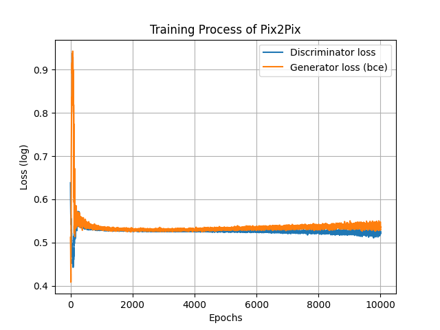
另外L1損失的部分會顯示生成器生成的圖片是否接近原圖,原則上這個損失要越低越好。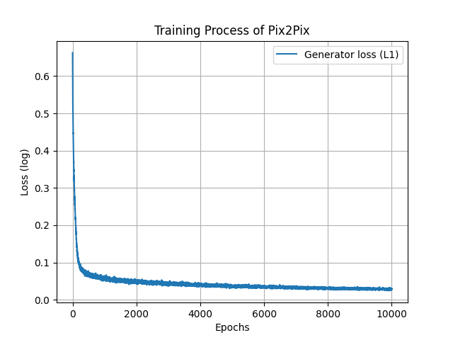
可以看得出來生成圖片有越來越接近原圖。
另外在訓練過程中我發現其實訓練大約200次的時候圖片基本就成形了,所以這邊會放上訓練更初期的變化給各位看看~
Epoch=0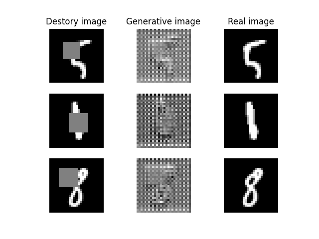
Epoch=10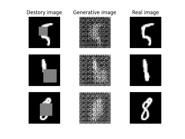
Epoch=20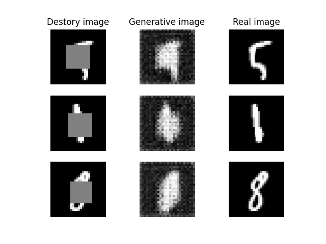
Epoch=70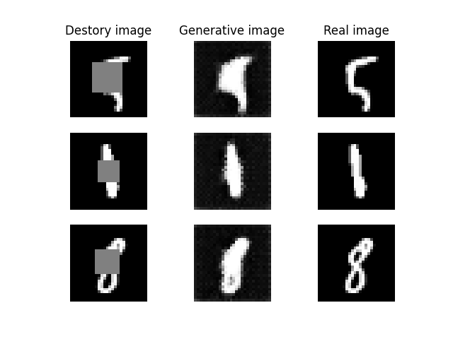
Epoch=200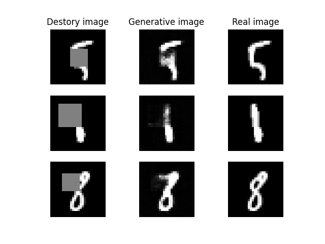
Epoch=1000,基本上後面生成就沒什麼進步了。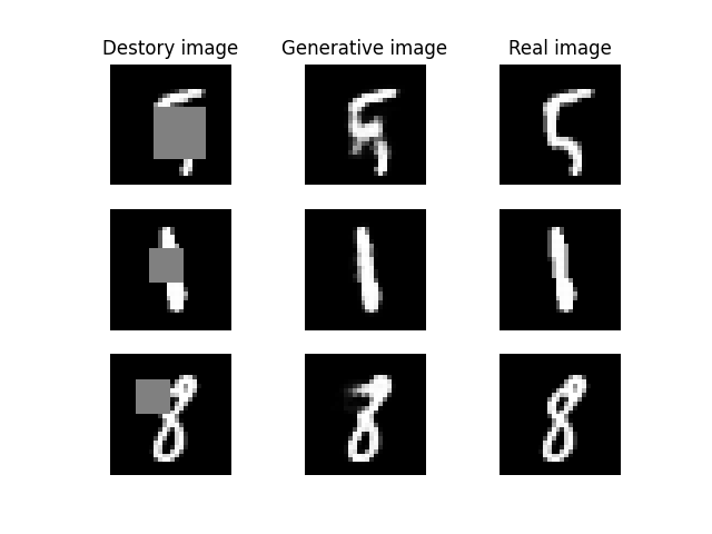
Epoch=10000,可以看到圖片有成功被修復。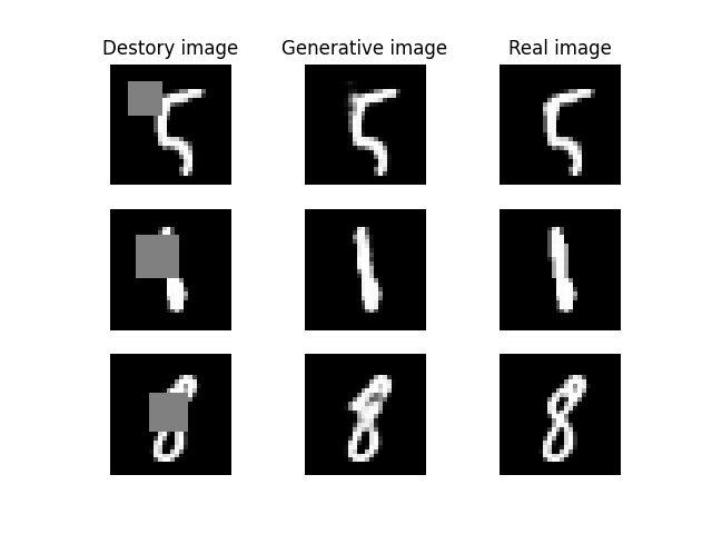
最後就是訓練過程的變化啦!
Pix2Pix是我剛入坑GAN時接觸的其中之一,剛開始理論與實作都給我帶來不少麻煩,不過寫了幾次後熟悉了它的運作原理後就沒那麼可怕了。我也覺得使用U-Net架構真的可以很好的處理圖片,之後要介紹的擴散模型也有使用U-Net,所以這個架構也要認識一下。明天會來介紹SRGAN,這也是一個很棒的GAN。今天的Pix2Pix各位也可以去試著挑戰其他應用!
from tensorflow.keras.datasets import mnist
from tensorflow.keras.layers import Input, BatchNormalization, LeakyReLU, Activation, Conv2DTranspose, Conv2D, Concatenate, Dropout
from tensorflow.keras.models import Model, save_model
from tensorflow.keras.optimizers import Adam
import matplotlib.pyplot as plt
import numpy as np
import os
from tensorflow.keras.utils import plot_model
from tensorflow.keras.losses import BinaryCrossentropy, MeanAbsoluteError

class Pix2Pix():
    def __init__(self, generator_lr, discriminator_lr):
        if not os.path.exists('./result/Pix2Pix/imgs'):
            os.makedirs('./result/Pix2Pix/imgs')

        self.generator_lr = generator_lr
        self.discriminator_lr = discriminator_lr
        #建立損失
        self.cross_entropy = BinaryCrossentropy(from_logits=True)
        self.l1 = MeanAbsoluteError()

        self.discriminator = self.build_discriminator()
        self.generator = self.build_generator()
        self.adversarial = self.build_adversarialmodel()
        #建立patcgGAN要判斷的圖片大小
        self.discriminator_patch = (7, 7, 1)
        self.gloss = []
        self.dloss = []

    def show_processed_image(self, img, processed_img):
        l_x_train = (processed_img + 1) / 2
        x_train = (img + 1) / 2
        fig, axs = plt.subplots(4, 4)
        count = 0
        axs[0, 0].set_title('Masked Image')
        axs[0, 1].set_title('Origin Image')
        axs[0, 2].set_title('Masked Image')
        axs[0, 3].set_title('Origin Image')
        for i in range(4):
            axs[i, 0].imshow(l_x_train[count, :, :, 0], cmap='gray')  # 毀損圖片
            axs[i, 0].axis('off')
            axs[i, 1].imshow(x_train[count, :, :, 0], cmap='gray')  # 生成圖片
            axs[i, 1].axis('off')
            axs[i, 2].imshow(l_x_train[count + 4, :, :, 0], cmap='gray')  # 毀損圖片
            axs[i, 2].axis('off')
            axs[i, 3].imshow(x_train[count + 4, :, :, 0], cmap='gray')  # 生成圖片
            axs[i, 3].axis('off')
            count += 1
        plt.show()
    def load_data(self):
        (x_train, _), (_, _) = mnist.load_data()
        x_train = x_train[:10000,:,:] #處理60000張照片比較久,故使用10000張照片就好
        x_train = (x_train / 127.5)-1
        x_train = x_train.reshape((-1, 28, 28, 1))
        destroy_x_train = x_train.copy() #要準備毀損的照片
        destroy_point = np.random.randint(low=3, high=15, size=(10000, )) #遮蔽地點的最左上角
        destroy_width = np.random.randint(low=8, high=13, size=(10000, )) #遮蔽面的寬度
        destroy_area = destroy_point+destroy_width #遮蔽地點的右下角
        #將每一張圖片根據其左上角到右下角建立一個灰色正方形的遮蔽部分
        for i in range(10000):
            #print進度
            print(f'\rDestroying the images... finish:{round(i/100,3)}%', end='')
            destroy_x_train[i, destroy_point[i]:destroy_area[i], destroy_point[i]:destroy_area[i], 0] = 0

        del destroy_point, destroy_width, destroy_area #刪除用不到的變數,節省記憶體空間
        # self.show_processed_image(img=x_train, processed_img=destroy_x_train)
        return x_train, destroy_x_train

    def build_generator(self):
        def UpSampling(input_, unit, kernel_size, strides=2, bn=True):
            #上採樣層使用ReLU
            x = Conv2DTranspose(unit, kernel_size=kernel_size, strides=strides, padding='same')(input_)
            x = Activation('relu')(x)
            if bn:
                x = BatchNormalization(momentum=0.8)(x)
            return x
        def DownSampling(input_, unit, kernel_size, strides=2, bn=True):
            #下採樣層使用LeakyReLU
            x = Conv2D(unit, kernel_size=kernel_size, strides=strides, padding='same')(input_)
            x = LeakyReLU(alpha=0.2)(x)
            if bn:
                x = BatchNormalization(momentum=0.8)(x)
            return x

        input_ = Input(shape=(28, 28, 1))
        #建立一個淺層的U-Net,要注意shape有沒有對上,這部分需要手動計算
        d1 = DownSampling(input_, unit=32, kernel_size=4, bn=False) #shape=(14,14,32)
        d2 = DownSampling(d1, unit=64, kernel_size=4) #shape=(7,7,64)
        latent = DownSampling(d2, unit=128, kernel_size=4, strides=1) #shape=(7,7,128)
        u1 = UpSampling(latent, unit=64, kernel_size=4, strides=1) #shape=(7,7,64)
        u1 = Concatenate(axis=-1)([u1, d2])
        u2 = UpSampling(u1, unit=32, kernel_size=4) #shape=(14,14,32)
        u2 = Concatenate(axis=-1)([u2, d1])
        out = Conv2DTranspose(1, kernel_size=4, strides=2, padding='same', activation='tanh')(u2)

        model = Model(inputs=input_, outputs=out, name='Generator')
        model.summary()
        plot_model(model=model,to_file='./result/Pix2Pix/Generator.png',show_shapes=True)
        return model

    def build_discriminator(self):
        def DownSampling(input_, unit, kernel_size, strides=2, bn=True):
            x = Conv2D(unit, kernel_size=kernel_size, strides=strides, padding='same')(input_)
            x = LeakyReLU(alpha=0.2)(x)
            if bn:
                x = BatchNormalization(momentum=0.8)(x)
            x = Dropout(0.3)(x)
            return x
        image_input = Input(shape=(28, 28, 1))
        destory_image_input = Input(shape=(28, 28, 1))
        input_ = Concatenate(axis=-1)([image_input, destory_image_input])

        x = DownSampling(input_, unit=32, kernel_size=4, bn=False)
        x = DownSampling(x, unit=64, kernel_size=4)
        out = Conv2D(1, kernel_size=4, strides=1, padding='same')(x)

        model = Model(inputs=[image_input, destory_image_input], outputs=out, name='Discriminator')
        dis_optimizer = Adam(learning_rate=self.discriminator_lr , beta_1=0.5)
        model.compile(loss=self.cross_entropy,
                      optimizer=dis_optimizer,
                      metrics=['accuracy'])
        model.summary()
        plot_model(model=model, to_file='./result/Pix2Pix/Discriminator.png', show_shapes=True)
        return model

    def build_adversarialmodel(self):
        #1.
        destory_image_input = Input(shape=(28, 28, 1))
        #2.
        generator_sample = self.generator(destory_image_input)
        #3
        self.discriminator.trainable = False
        out = self.discriminator([generator_sample, destory_image_input])
        #4
        model = Model(inputs=destory_image_input, outputs=[out, generator_sample])
        #5
        adv_optimizer = Adam(learning_rate=self.generator_lr, beta_1=0.5)
        model.compile(loss=[self.cross_entropy, self.l1], loss_weights=[1, 100], optimizer=adv_optimizer)
        plot_model(model=model, to_file='./result/Pix2Pix/Adversarial.png', show_shapes=True)
        model.summary()
        return model

    def train(self, epochs, batch_size=128, sample_interval=50):
        # 準備訓練資料
        x_train, destroy_x_train = self.load_data()
        #標籤要對照上使用PatchGAN的shape
        valid = np.ones((batch_size, ) + self.discriminator_patch)
        fake = np.zeros((batch_size, ) + self.discriminator_patch)
        for epoch in range(epochs):
            idx = np.random.randint(0, x_train.shape[0], batch_size)
            imgs = x_train[idx]
            destory_img = destroy_x_train[idx]
            gen_imgs = self.generator.predict(destory_img)
            #輸入別搞混了,別把遮擋圖與原圖給輸入相反了
            d_loss_real = self.discriminator.train_on_batch([imgs, destory_img], valid)
            d_loss_fake = self.discriminator.train_on_batch([gen_imgs, destory_img], fake)
            d_loss = 0.5 * np.add(d_loss_real, d_loss_fake)
            self.dloss.append(d_loss[0])
            #對抗模型訓練時要注意是要與真實標籤與真實圖去計算誤差
            g_loss = self.adversarial.train_on_batch(destory_img, [valid, imgs])
            self.gloss.append(g_loss)
            print(f"Epoch:{epoch} [D loss: {d_loss[0]:.4f}, acc: {100 * d_loss[1]:.2f}] [G loss: Total:{g_loss[0]:.4f}, crossentropy loss:{g_loss[1]:.4f}, L1 loss:{g_loss[2]:.6f}]")
            if epoch % sample_interval == 0:
                self.sample(epoch)
        self.save_data()
    def save_data(self):
        np.save(file='./result/Pix2Pix/generator_loss.npy',arr=np.array(self.gloss))
        np.save(file='./result/Pix2Pix/discriminator_loss.npy', arr=np.array(self.dloss))
        save_model(model=self.generator,filepath='./result/Pix2Pix/Generator.h5')
        save_model(model=self.discriminator,filepath='./result/Pix2Pix/Discriminator.h5')
        save_model(model=self.adversarial,filepath='./result/Pix2Pix/Adversarial.h5')

    def sample(self, epoch=None, num_images=9, save=True):
        r = int(np.sqrt(num_images))
        idx = [100, 200, 300] #手動隨機挑三張照片,比較好觀察變化
        x_train, destroy_x_train = self.load_data()
        destory_img = destroy_x_train[idx]
        x_train = x_train[idx]
        gen_imgs = self.generator.predict(destory_img)
        gen_imgs = (gen_imgs+1)/2
        fig, axs = plt.subplots(r, r)
        count = 0
        axs[0, 0].set_title('Destory image')
        axs[0, 1].set_title('Generative image')
        axs[0, 2].set_title('Real image')
        for i in range(r):
            axs[i, 0].imshow(destory_img[count, :, :, 0], cmap='gray')  #毀損圖片
            axs[i, 0].axis('off')
            axs[i, 1].imshow(gen_imgs[count, :, :, 0], cmap='gray') #生成圖片
            axs[i, 1].axis('off')
            axs[i, 2].imshow(x_train[count, :, :, 0], cmap='gray')  #真實圖片
            axs[i, 2].axis('off')
            count += 1
        if save:
            fig.savefig(f"./result/Pix2Pix/imgs/{epoch}epochs.png")
        else:
            plt.show()
        plt.close()

if __name__ == '__main__':
    gan = Pix2Pix(generator_lr=0.0002,discriminator_lr=0.0002)
    gan.train(epochs=10000, batch_size=64, sample_interval=200)
    gan.sample(save=False)