[Day23]：想把圖片轉高清圖？使用SRGAN吧

2023 iThome 鐵人賽

DAY 23

AI & Data

生成式AI到底何方神聖？一窺生程式AI的真面目系列第 23 篇

15th鐵人賽生成式ai 生成對抗網路 srgan 深度學習

golucky_sir

2023-09-26 00:15:41

454 瀏覽

分享至

前言

今天要來介紹SRGAN啦，這是一個可以把低解析度轉成高解析度圖片的應用，相信它一定非常實用吧，今天就來看看要如何建立SRGAN啦！

建立SRGAN模型

SRGAN模型需要使用VGG網路進行圖片特徵的萃取，不過VGG網路是只接受圖片長寬大於32且色彩通道必須為3的圖片。不過mnist都是長度為28，色彩通道為1的圖片，所以經過考慮後決定使用其他偷吃步的方法來取代VGG。不過效果一樣不差，所以還是可以使用。

第一步：決定任務類型與要使用的模型

這次任務是會使用低解析度的mnist (7, 7, 1)轉成原圖 (28, 28, 1)，使用SRGAN來訓練。

第二步：匯入函式庫

因為要處理圖片把圖片轉成低解析度的樣子，所以要使用OpenCV來處理。另外基本上SRGAN會使用VGG來計算感知損失，不過今天不會用到。因為VGG的輸入需要是彩色圖片且圖片大小也有限制，所以今天就使用別的模型來提取特徵，VGG的部分僅將匯入方法展示給各位看。

from tensorflow.keras.datasets import mnist
from tensorflow.keras.layers import Input, BatchNormalization, LeakyReLU, Conv2DTranspose, Conv2D, PReLU, Add, Dense
from tensorflow.keras.models import Model, save_model
from tensorflow.keras.optimizers import Adam
import matplotlib.pyplot as plt
import numpy as np
import os
import cv2 #匯入OpenCV
from tensorflow.keras.utils import plot_model
from tensorflow.keras.applications import VGG19 #匯入VGG模型，但這次不會用到

第三步：資料前處理 (Data Preprocessing)

要將圖片降低成低解析度的圖片也很簡單，只要使用cv2.resize()就好，最終效果如下：

cv2.resize()用法為：new_img = cv2.resize(img, (img_w, img_h), interpolation=插值方法)。img是原圖；(img_w, img_h)是縮放後的圖片長寬；interpolation是插植方法，插值方法參數設定如下表：

cv2.INTER_LINEAR	雙線性插值 (預設)
cv2.INTER_NEAREST	最近鄰插值
cv2.INTER_CUBIC	4*4像素鄰近使用三次插值
cv2.INTER_LANCZOS4	8*8像素鄰近使用的Lanczos插值
cv2.INTER_AREA	使用像素之間的區域關係重新採樣，今天會使用這個方法！

今天會使用cv2.INTER_AREA插值方法，各位有興趣也可以試試看其他插值法。若對插值法原理不理解的話也可以再去搜尋看看！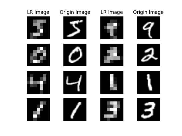

以下是資料處理完整的程式部份

def load_data(self,used_data_num=10000):
        (x_train, _), (_, _) = mnist.load_data()
        x_train = x_train[:used_data_num,:,:] #處理60000張照片比較久，故使用10000張照片就好
        x_train = (x_train / 127.5)-1
        x_train = x_train.reshape((-1, 28, 28, 1))
        #先處理第一張照片，之後的照片再用迴圈一筆一筆添加，否則在空的array中直接append shape會跑掉
        #處理完的shape是(7,7)
        lr_x_train = cv2.resize(x_train[0], (7, 7), interpolation=cv2.INTER_AREA).reshape((1,7,7,1))
        for i in range(1, used_data_num):
            print(f'\rDestroying the images... finish：{round(i/100,3)}%', end='')
            img = cv2.resize(x_train[i], (7, 7), interpolation=cv2.INTER_AREA)
            lr_x_train = np.append(arr=lr_x_train, values=img.reshape(1,7,7,1), axis=0)
        self.show_processed_image(img=x_train, processed_img=lr_x_train)
        return x_train, lr_x_train

另外也有展示圖片經過處理後的結果，這部分跟前天的Pix2Pix類似：

def show_processed_image(self, img, processed_img):
        l_x_train = (processed_img + 1) / 2
        x_train = (img + 1) / 2
        fig, axs = plt.subplots(4, 4)
        count = 0
        axs[0, 0].set_title('LR Image')
        axs[0, 1].set_title('Origin Image')
        axs[0, 2].set_title('LR Image')
        axs[0, 3].set_title('Origin Image')
        for i in range(4):
            axs[i, 0].imshow(l_x_train[count, :, :, 0], cmap='gray')  # 低解析度圖片
            axs[i, 0].axis('off')
            axs[i, 1].imshow(x_train[count, :, :, 0], cmap='gray')  # 原始圖片
            axs[i, 1].axis('off')
            axs[i, 2].imshow(l_x_train[count + 4, :, :, 0], cmap='gray')  # 低解析度圖片
            axs[i, 2].axis('off')
            axs[i, 3].imshow(x_train[count + 4, :, :, 0], cmap='gray')  # 原始圖片
            axs[i, 3].axis('off')
            count += 1
        plt.show()

第四步：建立生成模型類別

接下來就要來建立SRGAN了，經過幾次實驗以後發現SRGAN也使用類似PatchGAN的方式訓練效果會更不錯，所以SRGAN的判別器也會判斷許多小圖片。

在判別器建立時會動一點歪腦筋，使用判別器的"部分網路"作為特徵提取 (Feature Net)的網路，程式碼中是self.fn，這個網路會取代VGG用於計算感知損失。

class SRGAN():
    def __init__(self, generator_lr, discriminator_lr):
        if not os.path.exists('./result/SRGAN/imgs'):
            os.makedirs('./result/SRGAN/imgs')
        self.generator_lr = generator_lr
        self.discriminator_lr = discriminator_lr
				
		#建立判別器與特徵提取(fn)的網路
        self.discriminator, self.fn = self.build_discriminator()
        self.generator = self.build_generator()
        self.adversarial = self.build_adversarialmodel()

        self.discriminator_patch = (7, 7, 1)
        self.gloss = []
        self.dloss = []

第五步：建立模型、定義訓練方法

接著就要來定義模型了，SRGAN的作者很貼心給了網路架構的完整圖，但是我們的圖片並不會太大，所以也會適當的降低模型的層數與參數量。

生成器：生成器根據原始論文描述使用PReLU，並使用一些殘差區塊 (Residual Block)，殘差區塊使用卷積-批次正規化-PReLU-卷積-批次正規化BN-跳接組成。

來複習一下昨天原始論文提及到的模型架構，我將殘差簡化到剩兩個，神經元參數量與卷積核大小都有縮小，下方的C1、r、C2、x可以對照到程式碼範例中我定義的網路層：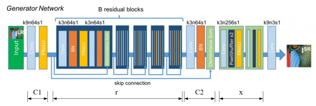

def build_generator(self):
        def UpSampling(input_, unit, kernel_size, strides=2):
            x = Conv2DTranspose(unit, kernel_size=kernel_size, strides=strides, padding='same')(input_)
            x = PReLU()(x)
            return x
        def Residual_Block(input_, unit):
            x = Conv2D(unit, kernel_size=2, strides=1, padding='same')(input_)
            x = BatchNormalization(momentum=0.8)(x)
            x = PReLU()(x)
            x = Conv2D(unit, kernel_size=2, strides=1, padding='same')(x)
            x = BatchNormalization(momentum=0.8)(x)
            x = Add()([x, input_])
            return x

        input_ = Input(shape=(7, 7, 1))
        c1 = Conv2D(32, kernel_size=3, strides=1, padding='same')(input_)
        c1 = PReLU()(c1)
        r = Residual_Block(c1, 32)
        r = Residual_Block(r, 32)
        c2 = Conv2D(32, kernel_size=2, strides=1, padding='same')(r)
        c2 = PReLU()(c2) #後來發現這層應該是BN，但訓練效果也還不錯
        c2 = Add()([c2, c1])
        x = UpSampling(c2, 64, kernel_size=2)
        x = UpSampling(x, 64, kernel_size=2)
        out = Conv2DTranspose(1, kernel_size=2, strides=1, padding='same', activation='tanh')(x)

        model = Model(inputs=input_, outputs=out, name='Generator')
        model.summary()
        plot_model(model=model,to_file='./result/SRGAN/Generator.png',show_shapes=True)
        return model

生成器網路架構圖如下，一樣使用plot_model()方法繪出的：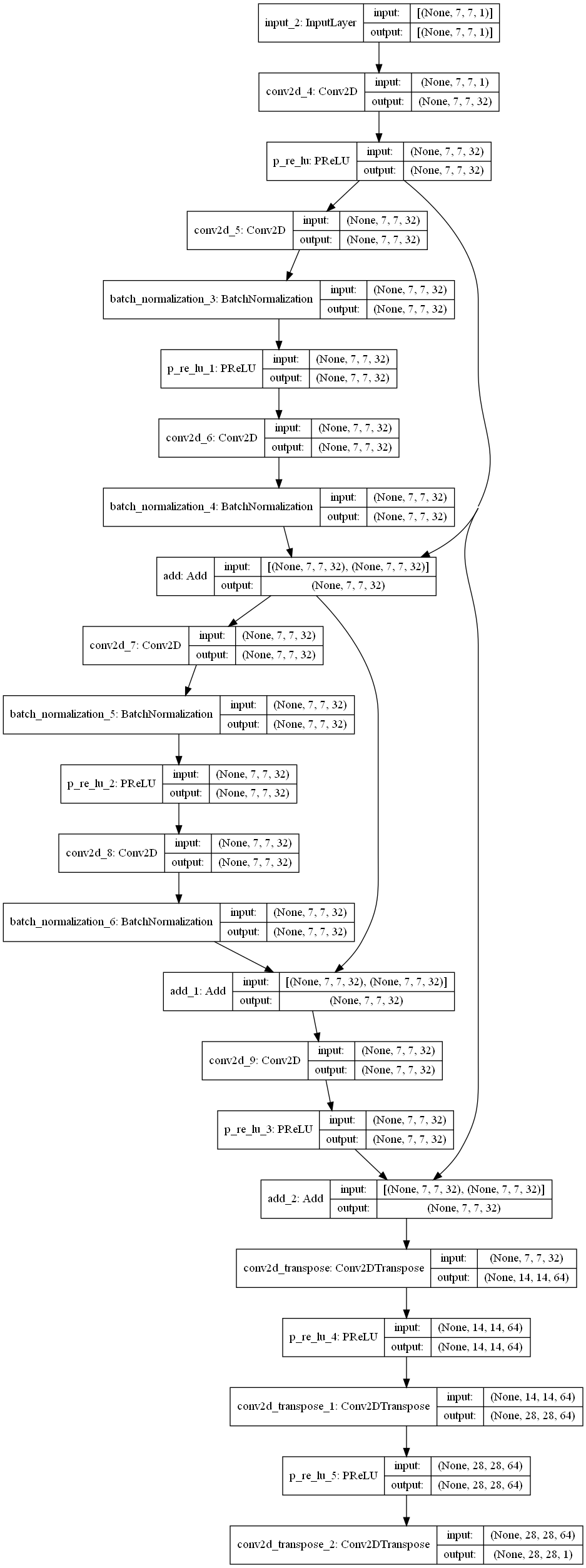

判別器：接著來看看判別器，判別器很簡單就是卷積-批次正規化BN-LeakyReLU結合的 (第一層沒有使用BN)，經過幾層後直接接到全連接層然後一個LeakyReLU再使用一個全連接層+sigmoid做輸出。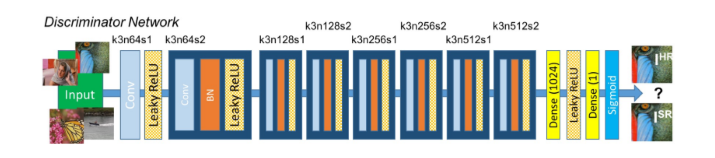

根據論文，我們可以適時做些修改並建立模型，以更符合實際任務需求。這邊我們發現經過下採樣三次後有一個feature，那是作為特徵提取網路用的輸出，經過了四個下採樣後得到的特徵就是圖片的特徵圖，我們將輸入層與feature額外作為一個模型，這個模型不用特別編譯。就算未經訓練，他的參數計算對於假圖或者真圖來說都是公平的，不會因為今天輸入假圖，參數就會變動等等。

接著判別器就正常建立並編譯就好了，最後要返回兩個模型分別是判別器與特徵提取網路以供訓練使用。

不過此方法在訓練圖片大一點的資料集就幾乎沒用了。所以使用解析度大一點的圖片還是要使用VGG模型來提取特徵喔。

def build_discriminator(self):
        def DownSampling(input_, unit, kernel_size, strides=1, bn=True):
            x = Conv2D(unit, kernel_size=kernel_size, strides=strides, padding='same')(input_)
            x = LeakyReLU(alpha=0.2)(x)
            if bn:
                x = BatchNormalization(momentum=0.8)(x)
            return x

        input_ = Input(shape=(28, 28, 1))
        x = DownSampling(input_, unit=32, kernel_size=2, bn=False)
        x = DownSampling(x, unit=32, kernel_size=2, strides=2)
        x = DownSampling(x, unit=64, kernel_size=2)
        feature = DownSampling(x, unit=64, kernel_size=2, strides=2) #特徵網路的輸出，是為取代VGG網路用的
        x = Dense(128)(feature)
        x = LeakyReLU(alpha=0.2)(x)
        out = Dense(1, activation='sigmoid')(x)

        fn_model = Model(inputs=input_, outputs=feature, name='fn') #取代VGG網路的特徵網路
        model = Model(inputs=input_, outputs=out, name='Discriminator')
        dis_optimizer = Adam(learning_rate=self.discriminator_lr , beta_1=0.5)
        model.compile(loss='mse',
                      optimizer=dis_optimizer,
                      metrics=['accuracy'])
        model.summary()
        plot_model(model=model, to_file='./result/SRGAN/Discriminator.png', show_shapes=True)
        return model, fn_model

編譯完模型後繪圖，下圖就是判別器模型的圖。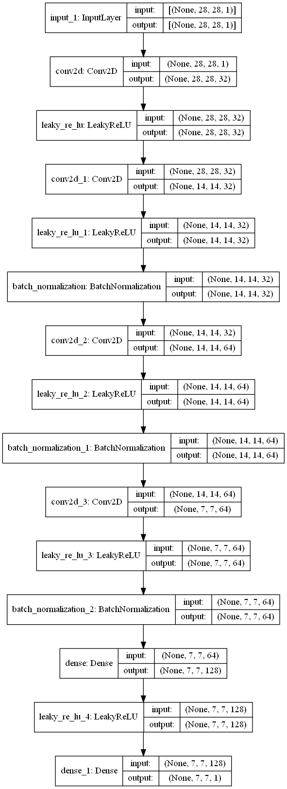

對抗模型：對抗模型建立上也沒有太複雜，只是也要將特徵圖作為輸出，好讓生成器可以比較感知損失。根據昨天介紹的SRGAN的目標函數，我們可以指定兩個損失函數的權重：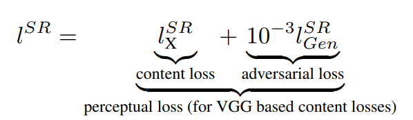

上式意思是總損失中，感知損失 (Contect loss, 使用MSE)加權為1；對抗損失 (Adversarial loss, 使用Binary CrossEntropy)加權為0.001。

def build_adversarialmodel(self):
        lr_image_input = Input(shape=(7, 7, 1))
        generator_sample = self.generator(lr_image_input)
        self.discriminator.trainable = False
        out = self.discriminator(generator_sample)
        #得到生成圖片的特徵(feature map)
        generator_sample_features = self.fn(generator_sample)
        model = Model(inputs=lr_image_input, outputs=[out, generator_sample_features])
        adv_optimizer = Adam(learning_rate=self.generator_lr, beta_1=0.5)
        model.compile(loss=['binary_crossentropy','mse'], loss_weights=[0.001, 1], optimizer=adv_optimizer)
        plot_model(model=model, to_file='./result/SRGAN/Adversarial.png', show_shapes=True)
        model.summary()
        return model

訓練步驟：訓練時與GAN差不多，只需要注意要記得提取真實圖片的特徵，並讓它作為對抗模型的答案，讓生成器訓練時也要去計算生成圖片的感知損失即可。基本上訓練都差不多是這樣，除了一些特定步驟要注意一下，GAN的訓練絕大部分都大同小異。

生成器訓練的損失有三個，第一個是損失加總、第二個是交叉熵 (未經過加權)、第三個是感知損失，即L2損失 (未經過加權)。

def train(self, epochs, batch_size=128, sample_interval=50):
        # 準備訓練資料
        x_train, lr_x_train= self.load_data()
        valid = np.ones((batch_size,) + self.discriminator_patch)
        fake = np.zeros((batch_size,) + self.discriminator_patch)
        for epoch in range(epochs):
            idx = np.random.randint(0, x_train.shape[0], batch_size)
            imgs = x_train[idx]
            lr_imgs = lr_x_train[idx]
            gen_imgs = self.generator.predict(lr_imgs)

            d_loss_real = self.discriminator.train_on_batch(imgs, valid)
            d_loss_fake = self.discriminator.train_on_batch(gen_imgs, fake)
            d_loss = 0.5 * np.add(d_loss_real, d_loss_fake)
            self.dloss.append(d_loss[0])
            image_features = self.fn(imgs) #使用特徵提取網路提取真實圖片的特徵
            g_loss = self.adversarial.train_on_batch(lr_imgs, [valid, image_features])
            self.gloss.append(g_loss)
            print(f"Epoch:{epoch} [D loss: {d_loss[0]}, acc: {100 * d_loss[1]:.2f}] [G loss: Total:{g_loss[0]:.4f}, crossentropy loss:{g_loss[1]:.4f}, L2 loss:{g_loss[2]:.6f}]")
            if epoch % sample_interval == 0:
                self.sample(epoch)
        self.save_data()

定義其他副程式

儲存資料的部分老樣子了：

def save_data(self):
        np.save(file='./result/SRGAN/generator_loss.npy',arr=np.array(self.gloss))
        np.save(file='./result/SRGAN/discriminator_loss.npy', arr=np.array(self.dloss))
        save_model(model=self.generator,filepath='./result/SRGAN/Generator.h5')
        save_model(model=self.discriminator,filepath='./result/SRGAN/Discriminator.h5')
        save_model(model=self.adversarial,filepath='./result/SRGAN/Adversarial.h5')

繪製訓練過程的程式碼也差不多就那樣，以低清圖-生成圖-真實圖去檢視生成圖片的進步。

def sample(self, epoch=None, num_images=9, save=True):
        r = int(np.sqrt(num_images))
        idx = [10, 20, 30] #手動隨機挑三張照片，比較好觀察變化
        x_train, lr_x_train = self.load_data(used_data_num=100)
        lr_x_train = lr_x_train[idx]
        x_train = x_train[idx]
        gen_imgs = self.generator.predict(lr_x_train)
        gen_imgs = (gen_imgs+1)/2
        fig, axs = plt.subplots(r, r)
        count = 0
        axs[0, 0].set_title('LR Image')
        axs[0, 1].set_title('Generative image')
        axs[0, 2].set_title('Real image')
        for i in range(r):
            axs[i, 0].imshow(lr_x_train[count, :, :, 0], cmap='gray')  #低清圖片
            axs[i, 0].axis('off')
            axs[i, 1].imshow(gen_imgs[count, :, :, 0], cmap='gray') #生成圖片
            axs[i, 1].axis('off')
            axs[i, 2].imshow(x_train[count, :, :, 0], cmap='gray')  #真實圖片
            axs[i, 2].axis('off')
            count += 1
        if save:
            fig.savefig(f"./result/SRGAN/imgs/{epoch}epochs.png")
        else:
            plt.show()
        plt.close()

第六步：開始訓練

訓練時我發現大概3000次訓練就可以訓練完成了，速度相當快：
超參數設定的部分如下表：

參數	參數值
生成器學習率	0.0002
判別器學習率	0.0002
Batch Size	64
訓練次數	3000

if __name__ == '__main__':
    gan = SRGAN(generator_lr=0.0002,discriminator_lr=0.0002)
    gan.train(epochs=3000, batch_size=64, sample_interval=200)
    gan.sample(save=False)

第七步：審視訓練結果並改進

來看看訓練的損失吧，可以看到生成器損失震盪非常大，但這不影響生成器生圖的品質。我們可以看到L2損失那條綠色的線也逐漸降低，雖然有一些震盪，但整體明顯有感覺到收斂。大概100多次訓練後L2損失才開始降低，那時候生成圖片的品質才開始變好。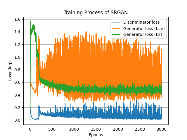

接著就來看看訓練過程吧，因為SRGAN訓練次數較少，所以會著重在前幾次的圖片生成，讓各位觀察看看訓練的變化。

Epoch=20，雜訊。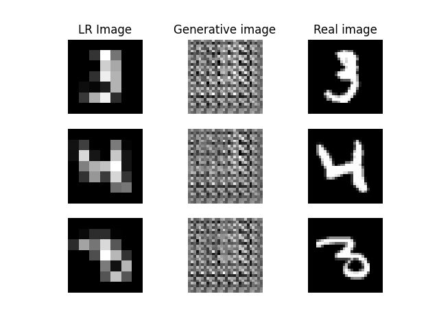

Epoch=100，有輪廓，但不多。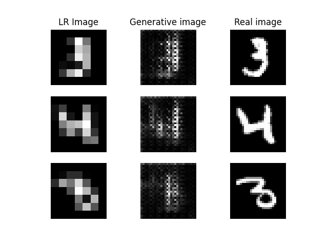

Epoch=200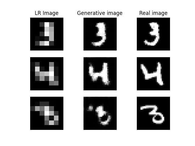

Epoch=1000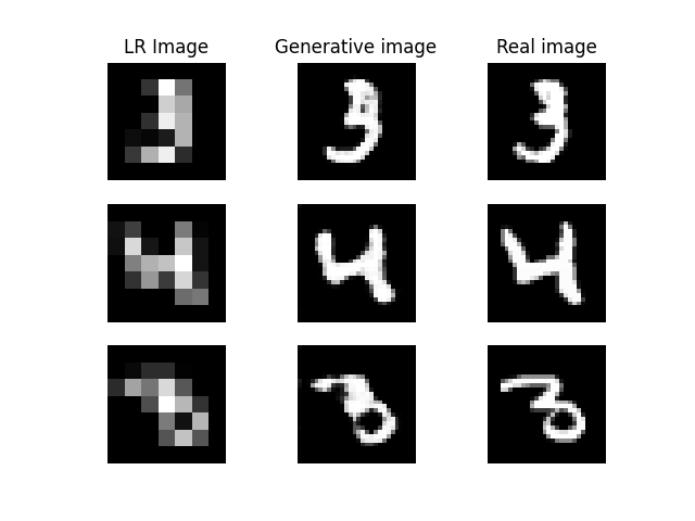

Epoch=3000，其實已經很不錯了。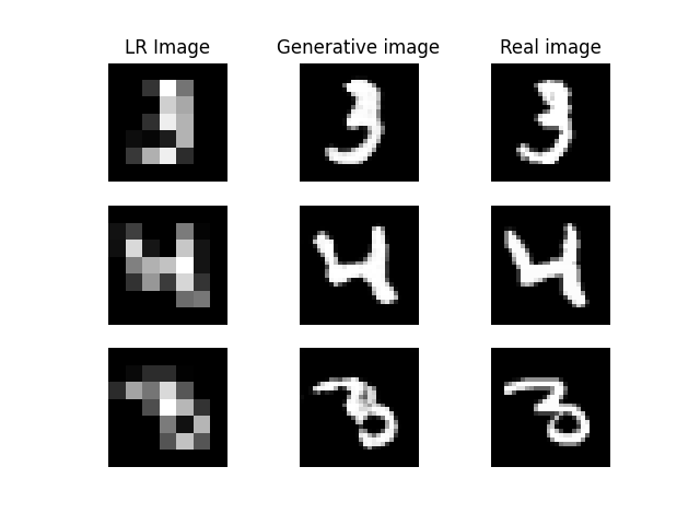

最後也是給各位看看生成圖片的變化，我覺得還蠻好看的：
SRGAN

結語

今天帶個為時做了SRGAN，原則上GAN的實作就到此為止了。明天會介紹其他的GAN，各位有時間的話也可以去實作看看那些GAN，基本上我在建立GAN的流程就不外乎是這幾步了。若各位對GAN的建立還沒有甚麼概念的話也歡迎參考我其他文章喔！

附錄：完整程式

from tensorflow.keras.datasets import mnist
from tensorflow.keras.layers import Input, BatchNormalization, LeakyReLU, Conv2DTranspose, Conv2D, PReLU, Add, Dense
from tensorflow.keras.models import Model, save_model
from tensorflow.keras.optimizers import Adam
import matplotlib.pyplot as plt
import numpy as np
import os
import cv2 #匯入OpenCV
from tensorflow.keras.utils import plot_model
from tensorflow.keras.applications import VGG19 #匯入VGG模型，但這次不會用到

class SRGAN():
    def __init__(self, generator_lr, discriminator_lr):
        if not os.path.exists('./result/SRGAN/imgs'):
            os.makedirs('./result/SRGAN/imgs')
        self.generator_lr = generator_lr
        self.discriminator_lr = discriminator_lr

        self.discriminator, self.fn = self.build_discriminator()
        self.generator = self.build_generator()
        self.adversarial = self.build_adversarialmodel()

        self.discriminator_patch = (7, 7, 1)
        self.gloss = []
        self.dloss = []

    def show_processed_image(self, img, processed_img):
        l_x_train = (processed_img + 1) / 2
        x_train = (img + 1) / 2
        fig, axs = plt.subplots(4, 4)
        count = 0
        axs[0, 0].set_title('LR Image')
        axs[0, 1].set_title('Origin Image')
        axs[0, 2].set_title('LR Image')
        axs[0, 3].set_title('Origin Image')
        for i in range(4):
            axs[i, 0].imshow(l_x_train[count, :, :, 0], cmap='gray')  # 低解析度圖片
            axs[i, 0].axis('off')
            axs[i, 1].imshow(x_train[count, :, :, 0], cmap='gray')  # 原始圖片
            axs[i, 1].axis('off')
            axs[i, 2].imshow(l_x_train[count + 4, :, :, 0], cmap='gray')  # 低解析度圖片
            axs[i, 2].axis('off')
            axs[i, 3].imshow(x_train[count + 4, :, :, 0], cmap='gray')  # 原始圖片
            axs[i, 3].axis('off')
            count += 1
        plt.show()
    def load_data(self,used_data_num=10000):
        (x_train, _), (_, _) = mnist.load_data()
        x_train = x_train[:used_data_num,:,:] #處理60000張照片比較久，故使用10000張照片就好
        x_train = (x_train / 127.5)-1
        x_train = x_train.reshape((-1, 28, 28, 1))
        #先處理第一張照片，之後的照片再用迴圈一筆一筆添加，否則在空的array中直接append shape會跑掉
        #處理完的shape是(7,7)
        lr_x_train = cv2.resize(x_train[0], (7, 7), interpolation=cv2.INTER_AREA).reshape((1,7,7,1))
        for i in range(1, used_data_num):
            print(f'\rDestroying the images... finish：{round(i/100,3)}%', end='')
            img = cv2.resize(x_train[i], (7, 7), interpolation=cv2.INTER_AREA)
            lr_x_train = np.append(arr=lr_x_train, values=img.reshape(1,7,7,1), axis=0)
        self.show_processed_image(img=x_train, processed_img=lr_x_train)
        return x_train, lr_x_train

    def build_generator(self):
        def UpSampling(input_, unit, kernel_size, strides=2):
            x = Conv2DTranspose(unit, kernel_size=kernel_size, strides=strides, padding='same')(input_)
            x = PReLU()(x)
            return x
        def Residual_Block(input_, unit):
            x = Conv2D(unit, kernel_size=2, strides=1, padding='same')(input_)
            x = BatchNormalization(momentum=0.8)(x)
            x = PReLU()(x)
            x = Conv2D(unit, kernel_size=2, strides=1, padding='same')(x)
            x = BatchNormalization(momentum=0.8)(x)
            x = Add()([x, input_])
            return x

        input_ = Input(shape=(7, 7, 1))
        c1 = Conv2D(32, kernel_size=3, strides=1, padding='same')(input_)
        c1 = PReLU()(c1)
        r = Residual_Block(c1, 32)
        r = Residual_Block(r, 32)
        c2 = Conv2D(32, kernel_size=2, strides=1, padding='same')(r)
        c2 = PReLU()(c2) #後來發現這層應該是BN，但訓練效果也還不錯
        c2 = Add()([c2, c1])
        x = UpSampling(c2, 64, kernel_size=2)
        x = UpSampling(x, 64, kernel_size=2)
        out = Conv2DTranspose(1, kernel_size=2, strides=1, padding='same', activation='tanh')(x)

        model = Model(inputs=input_, outputs=out, name='Generator')
        model.summary()
        plot_model(model=model,to_file='./result/SRGAN/Generator.png',show_shapes=True)
        return model

    def build_discriminator(self):
        def DownSampling(input_, unit, kernel_size, strides=1, bn=True):
            x = Conv2D(unit, kernel_size=kernel_size, strides=strides, padding='same')(input_)
            x = LeakyReLU(alpha=0.2)(x)
            if bn:
                x = BatchNormalization(momentum=0.8)(x)
            return x

        input_ = Input(shape=(28, 28, 1))
        x = DownSampling(input_, unit=32, kernel_size=2, bn=False)
        x = DownSampling(x, unit=32, kernel_size=2, strides=2)
        x = DownSampling(x, unit=64, kernel_size=2)
        feature = DownSampling(x, unit=64, kernel_size=2, strides=2) #特徵網路的輸出，是為取代VGG網路用的
        x = Dense(128)(feature)
        x = LeakyReLU(alpha=0.2)(x)
        out = Dense(1, activation='sigmoid')(x)

        fn_model = Model(inputs=input_, outputs=feature, name='fn') #取代VGG網路的特徵網路
        model = Model(inputs=input_, outputs=out, name='Discriminator')
        dis_optimizer = Adam(learning_rate=self.discriminator_lr , beta_1=0.5)
        model.compile(loss='mse',
                      optimizer=dis_optimizer,
                      metrics=['accuracy'])
        model.summary()
        plot_model(model=model, to_file='./result/SRGAN/Discriminator.png', show_shapes=True)
        return model, fn_model

    def build_adversarialmodel(self):
        lr_image_input = Input(shape=(7, 7, 1))
        generator_sample = self.generator(lr_image_input)
        self.discriminator.trainable = False
        out = self.discriminator(generator_sample)
        #得到生成圖片的特徵(feature map)
        generator_sample_features = self.fn(generator_sample)
        model = Model(inputs=lr_image_input, outputs=[out, generator_sample_features])
        adv_optimizer = Adam(learning_rate=self.generator_lr, beta_1=0.5)
        model.compile(loss=['binary_crossentropy','mse'], loss_weights=[0.001, 1], optimizer=adv_optimizer)
        plot_model(model=model, to_file='./result/SRGAN/Adversarial.png', show_shapes=True)
        model.summary()
        return model

    def train(self, epochs, batch_size=128, sample_interval=50):
        # 準備訓練資料
        x_train, lr_x_train= self.load_data()
        valid = np.ones((batch_size,) + self.discriminator_patch)
        fake = np.zeros((batch_size,) + self.discriminator_patch)
        for epoch in range(epochs):
            idx = np.random.randint(0, x_train.shape[0], batch_size)
            imgs = x_train[idx]
            lr_imgs = lr_x_train[idx]
            gen_imgs = self.generator.predict(lr_imgs)

            d_loss_real = self.discriminator.train_on_batch(imgs, valid)
            d_loss_fake = self.discriminator.train_on_batch(gen_imgs, fake)
            d_loss = 0.5 * np.add(d_loss_real, d_loss_fake)
            self.dloss.append(d_loss[0])
            image_features = self.fn(imgs) #使用特徵提取網路提取真實圖片的特徵
            g_loss = self.adversarial.train_on_batch(lr_imgs, [valid, image_features])
            self.gloss.append(g_loss)
            print(f"Epoch:{epoch} [D loss: {d_loss[0]}, acc: {100 * d_loss[1]:.2f}] [G loss: Total:{g_loss[0]:.4f}, crossentropy loss:{g_loss[1]:.4f}, L2 loss:{g_loss[2]:.6f}]")
            if epoch % sample_interval == 0:
                self.sample(epoch)
        self.save_data()
    def save_data(self):
        np.save(file='./result/SRGAN/generator_loss.npy',arr=np.array(self.gloss))
        np.save(file='./result/SRGAN/discriminator_loss.npy', arr=np.array(self.dloss))
        save_model(model=self.generator,filepath='./result/SRGAN/Generator.h5')
        save_model(model=self.discriminator,filepath='./result/SRGAN/Discriminator.h5')
        save_model(model=self.adversarial,filepath='./result/SRGAN/Adversarial.h5')

    def sample(self, epoch=None, num_images=9, save=True):
        r = int(np.sqrt(num_images))
        idx = [10, 20, 30] #手動隨機挑三張照片，比較好觀察變化
        x_train, lr_x_train = self.load_data(used_data_num=100)
        lr_x_train = lr_x_train[idx]
        x_train = x_train[idx]
        gen_imgs = self.generator.predict(lr_x_train)
        gen_imgs = (gen_imgs+1)/2
        fig, axs = plt.subplots(r, r)
        count = 0
        axs[0, 0].set_title('LR Image')
        axs[0, 1].set_title('Generative image')
        axs[0, 2].set_title('Real image')
        for i in range(r):
            axs[i, 0].imshow(lr_x_train[count, :, :, 0], cmap='gray')  #低清圖片
            axs[i, 0].axis('off')
            axs[i, 1].imshow(gen_imgs[count, :, :, 0], cmap='gray') #生成圖片
            axs[i, 1].axis('off')
            axs[i, 2].imshow(x_train[count, :, :, 0], cmap='gray')  #真實圖片
            axs[i, 2].axis('off')
            count += 1
        if save:
            fig.savefig(f"./result/SRGAN/imgs/{epoch}epochs.png")
        else:
            plt.show()
        plt.close()

if __name__ == '__main__':
    gan = SRGAN(generator_lr=0.0002,discriminator_lr=0.0002)
    gan.train(epochs=3000, batch_size=64, sample_interval=200)
    gan.sample(save=False)