一、介紹

在前一章節中，我們已經深入了解了邊緣檢測的基本原理，特別是與梯度運算和邊緣檢測的關聯性，以及一張圖片的邊緣在數學上的特性。OpenCV 提供了多種方法來實現邊緣檢測，每一種方法都有獨特的特性和適用情境。其中，較為常見的方法包括 Sobel 運算子、Scharr 運算子、Prewitt 運算子、Laplacian運算子，以及更高級的 Canny 邊緣檢測。

這些方法都是從圖片中捕捉出邊緣區域，進而突顯出影像中的物體結構和輪廓。然而，由於不同方法在計算梯度和處理邊緣的方式上存在差異，因此它們在實際應用中可能會有不同的表現，需要根據具體情況選擇最適合的方法。

二、 原理

1. 梯度向量的大小

上一章已經有講解過梯度的計算方式，在上一章中也提到梯度是一個向量，如果我們要得知某個x、y座標梯度的強度，需要使用下列的公式計算強度：

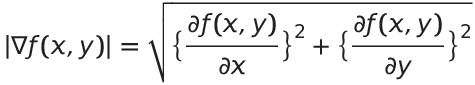
這個公式代表了在特定座標(x, y)處的梯度強度，分別對x和y方向上做偏微分，並將這兩個偏微分結果的平方相加，再取平方根，就能夠得到這個位置的梯度強度。通過對梯度強度的分析，我們可以找到影像中的強烈變化區域，進而識別出物體的邊緣。

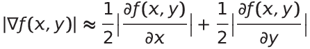
然而，對一張512x512圖片的每一個向量元素取出強度是蠻龐大的運算，開根號運算比起加法會花比較多的時間，畢竟開根號涉及更複雜的數學計算。為了節省開根號所耗費的時間，可以使用加法平均來近似開根號的結果，可以使用下列的公式近似：

2. 邊緣檢測運算子(Operator)

在進行邊緣檢測的過程中，我們需要使用特定的運算子。透過這些運算子對整張圖片進行摺積運算，我們能夠生成一個新的輪廓圖，這個輪廓圖可以用來突顯並提取影像中的輪廓。這個運算子的大小和內容將直接影響到邊緣檢測的結果。運算子的內容由一組權重構成，這些係數將與影像中相鄰像素的值進行加權總和，產生新的像素值。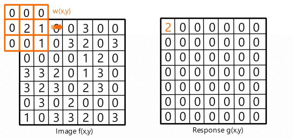

在邊緣檢測中，不同的運算子可以捕捉到不同方向和大小的邊緣特徵。以Sobel核和Prewitt核為例，它們是常見的邊緣檢測運算子，可以在水平和垂直方向上檢測出邊緣。而Laplacian核則更加敏感，能夠捕捉到更微小的變化，包括影像中的角點和紋理特徵。通過選擇適當的運算子，我們能夠有效地提取出不同類型的邊緣特徵，進一步幫助我們理解和分析影像的內容。

下圖是對一張原始圖片f(x,y)使用Sobel垂直運算子Wx(x,y) 進行摺積的過程。在這個過程中，我們可以看到原始圖片f(x,y)的元素與運算子Wx(x,y)進行元素相乘並加總的範例。可以看到原始圖片的垂直元素具有很大差異的灰階值，這會使原始圖片和核相乘加總取絕對值以後得到一個很大的值，這個值越大代表這個區塊是邊緣越有可能是邊緣。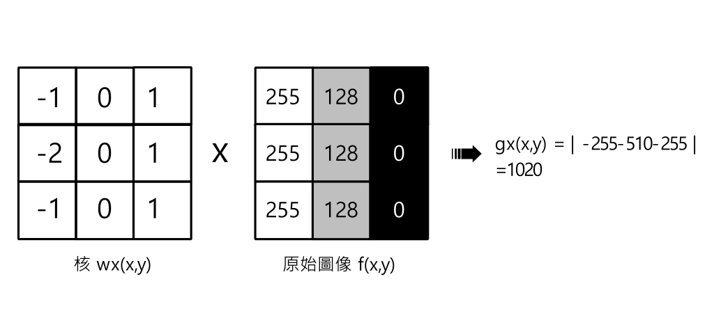

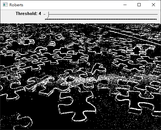
1) Roberts 運算子

Roberts邊緣檢測是一種簡單的邊緣檢測方法，用於識別影像中的邊緣區域。它使用兩個 2x2 的矩陣（稱為 Roberts 運算子）來計算影像的梯度，進而捕捉出強度變化的區域。Roberts運算子的結構和計算過程如下：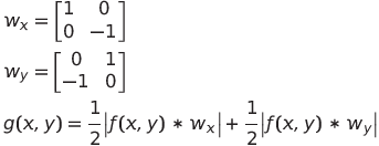

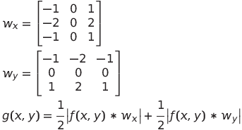
2) Sobel 運算子

Sobel運算子是一種常用於影像邊緣檢測的過濾器，用於捕捉影像中的強度變化，從而識別出物體的邊緣或輪廓。Sobel運算子通常在影像處理和計算機視覺中使用，它有助於檢測影像中的局部強度變化，從而找到物體的邊界。Sobel運算子可以計算每個像素的水平和垂直方向的梯度（變化率）。這些梯度可以用來識別影像中的亮度變化，進而找到邊緣位置。Sobel運算子的核心權重較簡單，計算複雜度相對較低，但在某些情況下可能對雜訊較敏感。Sobel運算子的結構和計算過程如下：

3) Scharr 運算子

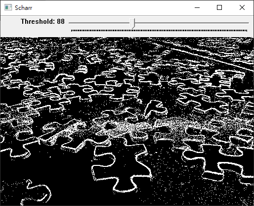
Scharr運算子是一種用於邊緣檢測的濾波器，它與Sobel運算子類似，但在計算梯度時更加敏感，檢測弱邊緣的能力較強。Scharr運算子的結構和計算過程如下：

4) Prewitt 運算子

Prewitt是一種邊緣檢測演算法，用於檢測影像中的邊緣特徵。Prewitt具有雜訊抑制的作用，可減少雜訊帶來的誤判。Prewitt運算子的結構和計算過程如下：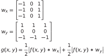

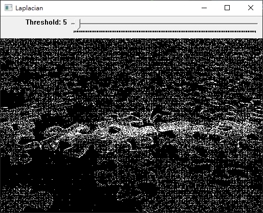
5) Laplacian 運算子

Laplacian（拉普拉斯）是一種在影像處理中廣泛使用的邊緣檢測算法。它不同於Sobel、Scharr、Prewitt等運算子，Laplacian是一種二階導數運算子，它在捕捉影像中的細微變化和邊緣更加敏感。

Laplacian運算子是一個中心值為正數，周圍值為負數或零的矩陣，用於對像素進行加權求和。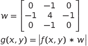

三、 程式碼

使用OpenCV的filter2D函示進行不同算法（Sobel、Roberts、Scharr、Prewitt、Laplacian）實現邊緣檢測。每個邊緣檢測函數的實現都包括使用filter2D函數進行摺積、轉換像素值到合適的範圍，以及最後的顯示過程。具體步驟如下：

1. 使用上述的運算子分別進行摺積。
2. 求出梯度向量的長度(或強度)。
3. 正規化讓值域位於0~255之間。
4. 使用二值化增強影像。

1. 逐行講解

1) 正規化

cv::normalize函數用於將影像數值正規化到指定的範圍內。這對於確保影像的亮度值在合適的範圍內。這行程式碼的作用是將scharr_dst影像的像素值經過正規化處理，使得像素值範圍落在0到255之間。這是為了確保影像的對比度和亮度在合適的範圍內，以便更好地顯示和後續處理。

cv::normalize(scharr_dst, scharr_dst,0, 255, cv::NormTypes::NORM_MINMAX);

參數的解釋如下：

1. src：輸入影像，你希望進行規範化的影像數值。
2. dst：輸出影像，規範化後的結果將被寫入這個影像。
3. 0：輸出影像的最小值，這裡設置為0。
4. 255：輸出影像的最大值，這裡設置為255，表示將像素值拉伸到0到255的範圍內。
5. cv::NormTypes::NORM_MINMAX：規範化的方式，這裡使用最小最大值範圍規範化，即將影像的最小值映射為0，最大值映射為255。

2) 加權平均

使用OpenCV的cv::addWeighted函數，用於將兩個影像進行加權相加，生成一個新的影像。這在影像處理中常用於合併或混合不同影像的效果。這行程式碼的作用是將兩個使用Scharr算子計算的水平和垂直梯度影像（scharr_dst_x和scharr_dst_y）進行加權相加，生成一個新的影像（scharr_dst）。

cv::addWeighted(scharr_dst_x, 0.5, scharr_dst_y, 0.5, 0, scharr_dst);

1. scharr_dst_x：第一個輸入影像，將會與第二個影像進行加權相加。
2. 0.5：第一個輸入影像的加權因子。這裡將第一個影像的像素值縮放為原來的一半。
3. scharr_dst_y：第二個輸入影像，將會與第一個影像進行加權相加。
4. 0.5：第二個輸入影像的加權因子。這裡將第二個影像的像素值縮放為原來的一半。
5. 0：Offset值，這將在兩個影像加權相加後被加到最終的結果上。
6. scharr_dst：輸出影像，加權相加後的結果將被寫入這個影像。

2. 完整程式碼

#include "opencv2/opencv.hpp"
#include "opencv2/core/utils/logger.hpp"

cv::Mat sobel(cv::Mat origin,int threshold);
cv::Mat roberts(cv::Mat origin,int threshold);
cv::Mat scharr(cv::Mat origin,int threshold);
cv::Mat prewitt(cv::Mat origin,int threshold);
cv::Mat laplacian(cv::Mat origin,int threshold);
cv::Mat grayImage;
void onSobel(int threshold, void*);
void onRoberts(int threshold, void*);
void onScharr(int threshold, void*);
void onPrewitt(int threshold, void*);
void onLaplacian(int threshold, void*);
int main()
{
	cv::utils::logging::setLogLevel(cv::utils::logging::LOG_LEVEL_ERROR);

	grayImage = cv::imread("C:\\Users\\vince\\Downloads\\puzzle.jpg",cv::IMREAD_GRAYSCALE);


	cv::namedWindow("Origin", cv::WINDOW_NORMAL);
	cv::resizeWindow("Origin", cv::Size(512,512*grayImage.rows/(float)grayImage.cols));

	cv::namedWindow("Sobel", cv::WINDOW_NORMAL);
	cv::resizeWindow("Sobel", cv::Size(512,512*grayImage.rows/(float)grayImage.cols));
	cv::createTrackbar("Threshold","Sobel", NULL, 255, onSobel);

	cv::namedWindow("Roberts", cv::WINDOW_NORMAL);
	cv::resizeWindow("Roberts", cv::Size(512,512*grayImage.rows/(float)grayImage.cols));
	cv::createTrackbar("Threshold","Roberts", NULL, 255,onRoberts);


	cv::namedWindow("Scharr", cv::WINDOW_NORMAL);
	cv::resizeWindow("Scharr", cv::Size(512,512*grayImage.rows/(float)grayImage.cols));
	cv::createTrackbar("Threshold","Scharr", NULL, 255,onScharr);

	cv::namedWindow("Prewitt", cv::WINDOW_NORMAL);
	cv::resizeWindow("Prewitt", cv::Size(512,512*grayImage.rows/(float)grayImage.cols));
	cv::createTrackbar("Threshold","Prewitt", NULL, 255,onPrewitt);

	cv::namedWindow("Laplacian", cv::WINDOW_NORMAL);
	cv::resizeWindow("Laplacian", cv::Size(512,512*grayImage.rows/(float)grayImage.cols));
	cv::createTrackbar("Threshold","Laplacian", NULL, 255,onLaplacian);
	cv::imshow("Origin", grayImage);


	cv::waitKey(0);
	return 0;
}

 
void onSobel(int threshold, void*) {
	cv::Mat dst = sobel(grayImage,threshold);
	cv::imshow("Sobel", dst);
}

void onRoberts(int threshold, void*) {
	cv::Mat dst = roberts(grayImage,threshold);
	cv::imshow("Roberts", dst);
}
void onScharr(int threshold, void*) {
	cv::Mat dst = scharr(grayImage,threshold);
	cv::imshow("Scharr", dst);
}
void onPrewitt(int threshold, void*) {
	cv::Mat dst = prewitt(grayImage,threshold);
	cv::imshow("Prewitt", dst);

}
void onLaplacian(int threshold, void*) {
	cv::Mat dst = laplacian(grayImage,threshold);
	cv::imshow("Laplacian", dst);
}


cv::Mat sobel(cv::Mat origin,int threshold) {
	cv::Mat sobel_dst_x;
	cv::Mat sobel_dst_y;
	cv::Mat sobel_dst;

	float kernel_data_x[9] = {-1,0,1,-2,0,2,-1,0,1};
	float kernel_data_y[9] = {-1,-2,-1,0,0,0,1,2,1};

	cv::Mat kernel_x = cv::Mat(3,3, CV_32F, kernel_data_x);
	cv::Mat kernel_y = cv::Mat(3,3, CV_32F,kernel_data_y);

	cv::filter2D(origin,sobel_dst_x,CV_32F,kernel_x);
	cv::convertScaleAbs(sobel_dst_x,sobel_dst_x);
	cv::filter2D(origin,sobel_dst_y,CV_32F,kernel_y);
	cv::convertScaleAbs(sobel_dst_y,sobel_dst_y);
	cv::addWeighted(sobel_dst_x, 0.5, sobel_dst_y, 0.5, 0, sobel_dst);
	
	cv::normalize(sobel_dst, sobel_dst,0, 255, cv::NormTypes::NORM_MINMAX);
	cv::Mat dst;
	cv::threshold(sobel_dst, dst, threshold, 255, cv::THRESH_BINARY);
	return dst;
}

cv::Mat roberts(cv::Mat origin,int threshold) {
	cv::Mat roberts_dst_x;
	cv::Mat roberts_dst_y;
	cv::Mat roberts_dst;

	float kernel_data_x[4] = {1,0,0,-1};
	float kernel_data_y[4] = {0,1,-1,0};
	cv::Mat kernel_x = cv::Mat(2,2, CV_32F, kernel_data_x);
	cv::Mat kernel_y = cv::Mat(2,2, CV_32F,kernel_data_y);

	cv::filter2D(origin,roberts_dst_x,CV_32F,kernel_x);
	cv::convertScaleAbs(roberts_dst_x,roberts_dst_x);

	cv::filter2D(origin,roberts_dst_y,CV_32F,kernel_y);
	cv::convertScaleAbs(roberts_dst_y,roberts_dst_y);

	cv::addWeighted(roberts_dst_x, 0.5, roberts_dst_y, 0.5, 0, roberts_dst);

	cv::normalize(roberts_dst_x, roberts_dst_x,0, 255, cv::NormTypes::NORM_MINMAX);
	cv::Mat dst;
	cv::threshold(roberts_dst, dst, threshold, 255, cv::THRESH_BINARY);
	return dst;
}

cv::Mat scharr(cv::Mat origin,int threshold) {
	cv::Mat scharr_dst_x;
	cv::Mat scharr_dst_y;
	cv::Mat scharr_dst;

	float kernel_data_x[9] = {-3,0,3,-10,0,10,-3,0,3};
	float kernel_data_y[9] = {-3,-10,-3,0,0,0,3,10,3};
	cv::Mat kernel_x = cv::Mat(3,3, CV_32F, kernel_data_x);
	cv::Mat kernel_y = cv::Mat(3,3, CV_32F,kernel_data_y);

	cv::filter2D(origin,scharr_dst_x,CV_32F,kernel_x);
	cv::convertScaleAbs(scharr_dst_x,scharr_dst_x);

	cv::filter2D(origin,scharr_dst_y,CV_32F,kernel_y);
	cv::convertScaleAbs(scharr_dst_y,scharr_dst_y);

	cv::addWeighted(scharr_dst_x, 0.5, scharr_dst_y, 0.5, 0, scharr_dst);

	cv::normalize(scharr_dst, scharr_dst,0, 255, cv::NormTypes::NORM_MINMAX);

	cv::Mat dst;
	cv::threshold(scharr_dst, dst, threshold, 255, cv::THRESH_BINARY);
	return dst;

}


cv::Mat prewitt(cv::Mat origin,int threshold) {
	cv::Mat prewitt_dst_x;
	cv::Mat prewitt_dst_y;
	cv::Mat prewitt_dst;

	float kernel_data_x[9] = {-1,0,1,-1,0,1,-1,0,1};
	float kernel_data_y[9] = {1,1,1,0,0,0,-1,-1,-1};
	cv::Mat kernel_x = cv::Mat(3,3, CV_32F, kernel_data_x);
	cv::Mat kernel_y = cv::Mat(3,3, CV_32F,kernel_data_y);

	cv::filter2D(origin,prewitt_dst_x,CV_32F,kernel_x);
	cv::convertScaleAbs(prewitt_dst_x,prewitt_dst_x);

	cv::filter2D(origin,prewitt_dst_y,CV_32F,kernel_y);
	cv::convertScaleAbs(prewitt_dst_y,prewitt_dst_y);

	cv::addWeighted(prewitt_dst_x, 0.5, prewitt_dst_y, 0.5, 0, prewitt_dst);

	cv::normalize(prewitt_dst, prewitt_dst,0, 255, cv::NormTypes::NORM_MINMAX);

	cv::Mat dst;
	cv::threshold(prewitt_dst, dst, threshold, 255, cv::THRESH_BINARY);
	return dst;

}

cv::Mat laplacian(cv::Mat origin,int threshold) {
	cv::Mat laplacian_dst;

	float kernel_data[9] = {0,-1,0,-1,4,-1,0,-1,0};
	cv::Mat kernel = cv::Mat(3,3, CV_32F, kernel_data);

	cv::filter2D(origin,laplacian_dst,CV_32F,kernel);
	cv::convertScaleAbs(laplacian_dst,laplacian_dst);

	cv::normalize(laplacian_dst, laplacian_dst,0, 255, cv::NormTypes::NORM_MINMAX);
	cv::Mat dst;
	cv::threshold(laplacian_dst, dst, threshold, 255, cv::THRESH_BINARY);
	return dst;

}

3. 測試結果

1) 原圖

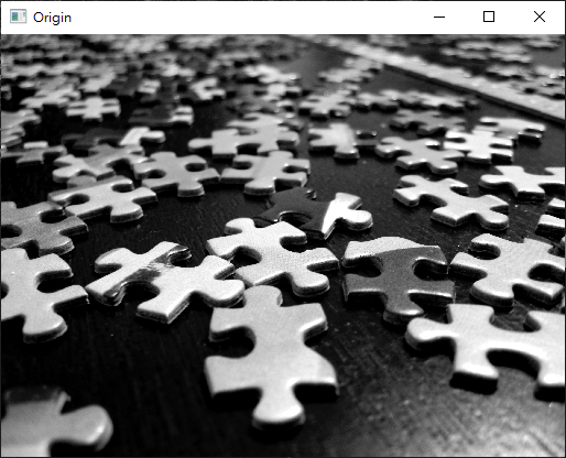
攝影師：Pixabay: https://www.pexels.com/zh-tw/photo/269399/

2) Sobel

使用Sobel濾波後觀察到邊緣清晰但同時有輕微雜訊的情況。

3) Roberts

使用Roberts濾波後觀察到相比起Sobel，有較多雜訊的情況。

4) Scharr

使用Scharr濾波後觀察到，弱邊緣變得更清晰但同時有明顯雜訊的情況，因此需要使用較大的閾值濾除雜訊。

5) Prewitt

使用Prewitt濾波後觀察到，Prewitt比Sobel濾波有更好的抗雜訊能力。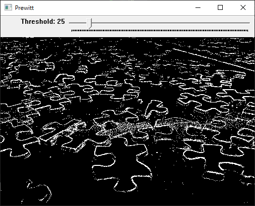

6) Laplacian

使用Laplacian濾波後觀察到，Laplacian很容易受到雜訊干擾。