
前面幾天已經介紹了不少和訓練有關的技巧啦,今天則是會來個大雜燴,把所有技巧全部串接起來做出一個訓練模型的流程,算是總複習!
但在訓練之前,當然先要有資料集啦,大部分的人都會使用 mnist 都做範例,但...我覺得有點氾濫這邊並不想XD,所以我們來自己產生訓練集吧!我自己使用 cv2 的 line、rectangle 和 circle 畫出 128x128 圖像,實作方法可以看 這裡 。
產生的圖片如圖: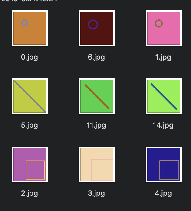
如果用原圖並不好訓練,所以我們複習一下 day12 的產生 tfrecord 方法。
def data_to_example(shape_type, type_index, image):
   example = tf.train.Example(features=tf.train.Features(feature={
       'shape/type': bytes_feature(shape_type.encode('utf8')),  # 存形狀
       'shape/type_index': int64_feature(type_index),  # 存編號
       'shape/image': bytes_feature(image),  # 存圖片
   }))
   return example
Line 的圖形編號: 0
Rectangle 的圖形編號: 1
Circle 的圖形編號: 2
就產生了 shape.tfrecord。
接下來回來看訓練的程式碼,我們定義的網路結構如下:
global_step = tf.train.get_or_create_global_step()
input_node = tf.placeholder(shape=[None, 128, 128, 3],
                           dtype=tf.float32,
                           name='input_node')
training_node = tf.placeholder_with_default(True,
                                           shape=(),
                                           name='training')
labels = tf.placeholder(shape=[None],
                       dtype=tf.int64,
                       name='img_labels')

with tf.variable_scope('backend'):
   net = tf.layers.conv2d(input_node, 32, (3, 3),
                          strides=(1, 1),
                          padding='same',
                          name='conv_1')
   net = tf.layers.batch_normalization(net,
                                       training=training_node,
                                       name='bn_1')
   net = tf.nn.relu6(net, name='relu_1')
   net = tf.layers.max_pooling2d(net, (2, 2),
                                 strides=(2, 2),
                                 name='max_pool_1')  # 64

   net = tf.layers.conv2d(net, 64, (3, 3),
                          strides=(1, 1),
                          padding='same',
                          name='conv_2')
   net = tf.layers.batch_normalization(net,
                                       training=training_node,
                                       name='bn_2')
   net = tf.nn.relu6(net, name='relu_2')
   net = tf.layers.dropout(net, 0.1,
                           training=training_node,
                           name='dropout_2')
   net = tf.layers.max_pooling2d(net, (2, 2),
                                 strides=(2, 2),
                                 name='max_pool_2')  # 32

   net = tf.layers.conv2d(net, 128, (3, 3),
                          strides=(2, 2),
                          padding='same',
                          name='conv_3')  # 16
   net = tf.layers.batch_normalization(net,
                                       training=training_node,
                                       name='bn_3')
   net = tf.nn.relu6(net, name='relu_3')
   net = tf.layers.max_pooling2d(net, (2, 2),
                                 strides=(2, 2),
                                 name='max_pool_3')  # 8

net = tf.reshape(net, [-1, 8 * 8 * 128], name='flatten')
logit = tf.layers.dense(net, 3, use_bias=False,
                       kernel_initializer=WEIGHT_INIT,
                       kernel_regularizer=REGULARIZER,
                       name='final_dense')
主要架構分成了三個部分,用到了 batch normalization 和 dropout (會這樣設計主要是方便後面幾天的講解),最後面先 flatten 後再接 dense layer 做分類判斷。
使用 day16 介紹到的 piecewise_constant 來改變 learning rate。
lr = tf.train.piecewise_constant(global_step,
                                boundaries=[250, 500, 750],
                                values=[0.1, 0.05, 0.01, 0.001],
                                name='lr_schedule')
另外 day18 時,我們透過 GraphKeys.REGULARIZATION_LOSSES 拿到權重的 loss 值。
with tf.variable_scope('loss'):
   inference_loss = tf.reduce_mean(
       tf.nn.sparse_softmax_cross_entropy_with_logits(
           logits=logit,
           labels=labels), name='inference_loss')
   wd_loss = tf.reduce_sum(
       tf.get_collection(tf.GraphKeys.REGULARIZATION_LOSSES),
                           name='wd_loss')
   total_loss = tf.add(inference_loss, wd_loss,
                           name='total_loss')

train_acc, acc_op = tf.metrics.accuracy(labels,
                                    tf.argmax(logit, 1),
                                    name='accuracy')
test_acc_node = tf.placeholder(dtype=tf.float32, shape=(),
                                    name='test_acc')
day20 我們詳細介紹了各種 Optimizer 的使用方法。
opt = tf.train.GradientDescentOptimizer(learning_rate=lr)
grads = opt.compute_gradients(total_loss)
update_ops = tf.get_collection(tf.GraphKeys.UPDATE_OPS)
with tf.control_dependencies(update_ops):
   train_op = opt.apply_gradients(grads, global_step=global_step)
day21 示範了如何使用 tf.summary 來記錄資料。
summary = tf.summary.FileWriter(OUTPUT_PATH, graph=tf.get_default_graph())
summaries = []

for grad, var in grads:
   if grad is not None:
       summaries.append(
           tf.summary.histogram(var.op.name + '/gradients', grad))

for var in tf.trainable_variables():
   summaries.append(tf.summary.histogram(var.op.name, var))

summaries.append(tf.summary.scalar('loss/total', total_loss))
summaries.append(tf.summary.scalar('loss/inference', inference_loss))
summaries.append(tf.summary.scalar('loss/weight', wd_loss))
summaries.append(tf.summary.scalar('accuracy/train', train_acc))
summaries.append(tf.summary.scalar('accuracy/test', test_acc_node))
summary_op = tf.summary.merge(summaries)
day19 介紹如何把目前模型狀態的資訊顯示出來。
total_parameters = 0
for variable in tf.get_collection(tf.GraphKeys.TRAINABLE_VARIABLES):
   shape = variable.get_shape()
   variable_parameters = 1
   for dim in shape:
       variable_parameters *= dim.value
   total_parameters += variable_parameters
print('trainable parameters count: %d' % total_parameters)
day14 展示怎麼使用 TFRecordDataset ,而在這邊我們分別宣告了訓練集和驗證集。
with tf.variable_scope('train_iterator'):
   data_set = tf.data.TFRecordDataset(TRAIN_TFRECORD_PATH)
   data_set = data_set.map(parse_function)
   data_set = data_set.batch(BATCH_SIZE)
   train_iterator = data_set.make_initializable_iterator()
   next_train_element = train_iterator.get_next()

with tf.variable_scope('test_iterator'):
   data_set = tf.data.TFRecordDataset(TEST_TFRECORD_PATH)
   data_set = data_set.map(parse_function)
   data_set = data_set.batch(BATCH_SIZE)
   test_iterator = data_set.make_initializable_iterator()
   next_test_element = test_iterator.get_next()
這邊的大雜燴,我們設定每 20 個 step 就紀錄一次跑一次驗證集,避免過擬合並且記錄 summary,之後就可以在 tensorboard 看到成果。
while True:
   try:
       labels_train, images_train = sess.run(next_train_element)
       if images_train.shape[0] != BATCH_SIZE:
           break

       _, total_loss_val, train_acc_val, current_step = \
           sess.run([train_op, total_loss, acc_op, global_step],
                    feed_dict={input_node: images_train,
                               labels: labels_train})

       print('step: %d, total_lost: %.2f, train_acc_val: %.2f' %
             (current_step, total_loss_val, train_acc_val))

       if current_step % 20 == 0:
           test_acc = eval_acc(sess, test_iterator, next_test_element,
                               logit, input_node, labels, training_node)
           summary_op_val = sess.run(summary_op,
                               feed_dict={input_node: images_train,
                                          labels: labels_train,
                                          test_acc_node: test_acc,
                                          training_node: False})
           print('test_acc: %.2f' % test_acc)
           summary.add_summary(summary_op_val, current_step)

   except tf.errors.OutOfRangeError:
       print('next epoch.')
       break  # epoch end
最後我最想強調的,養成產生 ckpt 的習慣,這樣如果訓練到一半程式當掉,至少你不用重頭開始。
saver.save(sess, "../ckpt/model.ckpt", global_step=global_step, latest_filename='shape_model')
好!程式執行後,我們就來觀察結果吧!
老樣子,第一個是 graph 的樣子。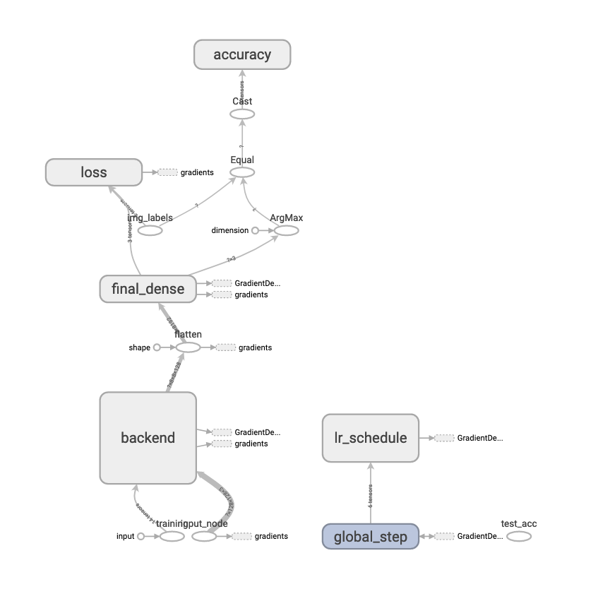
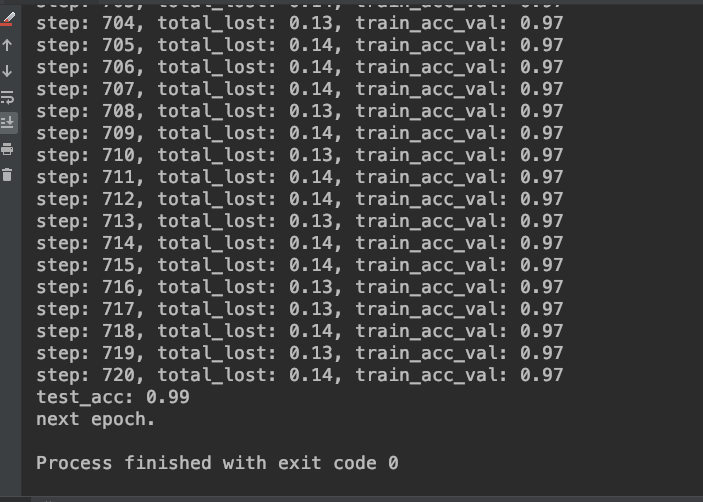
然後是訓練過程中 console 產生的訊息。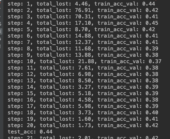
還有 accuracy 和 loss 的曲線圖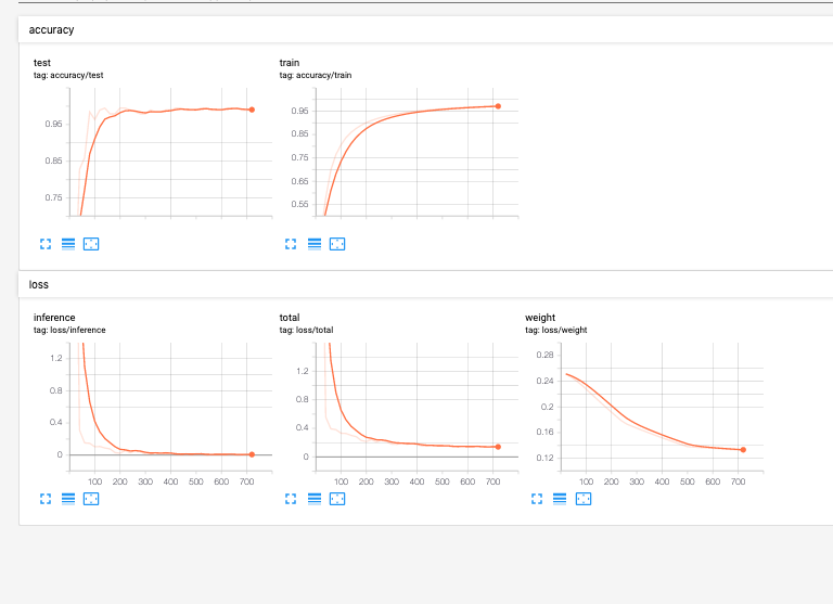
最後是觀察權重是否健康的 Histogram 。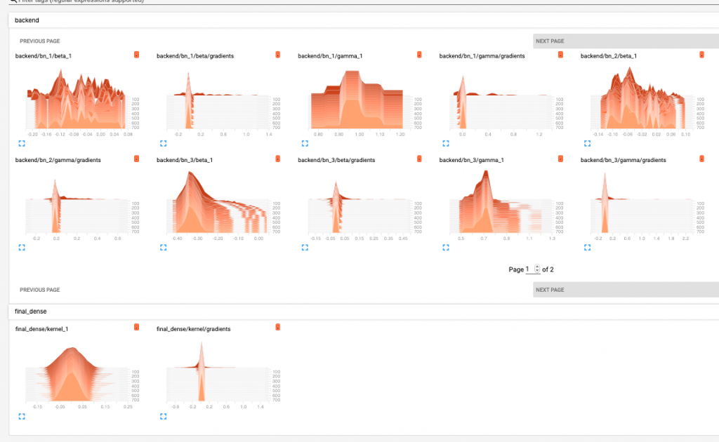
以上就是整個訓練過程的大雜燴,希望大家都能駕輕就熟!

 iThome鐵人賽