今日大綱

• 資料集
• Loss function
• 程式碼

資料集

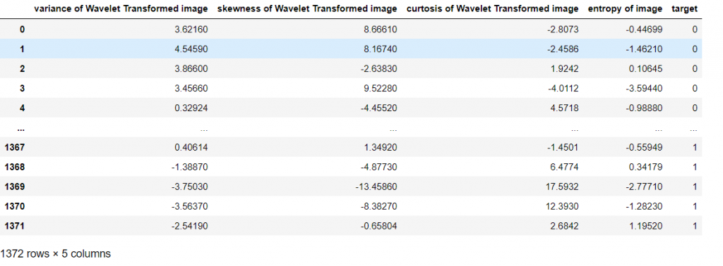
今天我所使用的資料集為UCI所提供的，其目的預測鈔票的真假。四個獨立變數皆為影像相關的變異數、標準差、偏態與不純度，皆為連續變數。

Loss function

Loss function很常與Cost function搞混，連我也會搞混，但這兩者是不同的東西，loss function計算單一樣本的誤差，而cost function為所有樣本誤差的平均值。
SVM的loss稱為hinge loss，公式如下:

如果預測正確，那麼預測值與實際值同號，損失值就是0；反之，如果預測錯誤，那麼就會有損失發生。

程式碼

首先，匯入資料集與指定欄位名稱。

import pandas as pd
url='https://archive.ics.uci.edu/ml/machine-learning-databases/00267/data_banknote_authentication.txt'
columns = ['variance of Wavelet Transformed image', 'skewness of Wavelet Transformed image', 'curtosis of Wavelet Transformed image', 'entropy of image', 'target']
data = pd.read_csv(url, names = columns)
data

將資料切成訓練集與測試集，分別為80%與20%，random state設置為1，其作用為固定每次取樣時一致。如果同一份資料集，不管何時測試，當random state一樣時，結果會一樣。

from sklearn.model_selection import train_test_split
from sklearn.svm import SVC
x = data.iloc[:,:-1]
y = data.iloc[:, -1]
x_train, x_test, y_train, y_test = train_test_split(x, y, test_size = 0.2, random_state = 1)

SVM的kernel function設為rbf，並且進行預測

svm = SVC(kernel='rbf')
svm.fit(x_train, y_train)
prediction = svm.predict(x_test)

將混淆矩陣視覺化

from sklearn.metrics import plot_confusion_matrix, classification_report
import matplotlib.pyplot as plt
color = 'black'
cm = plot_confusion_matrix(svm, x_test, y_test, cmap=plt.cm.Blues)
plt.title("Confusion matrix")
plt.xlabel("Predicted value", color = color)
plt.ylabel("Actual value", color = color)
plt.show()

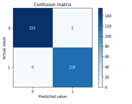
從圖可以發現有兩個樣本預測錯誤

檢視模型的precision、recall與accuracy

report = classification_report(y_test, prediction)
print(report)

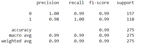
此模型的準確率高達0.99。

最後畫出模型的ROC，並且算出AUC

from sklearn.metrics import roc_curve, roc_auc_score, auc

# 在各種『決策門檻』（decision threshold）下，計算 『真陽率』（True Positive Rate；TPR）與『假陽率』（False Positive Rate；FPR）
fpr, tpr, threshold = roc_curve(y_test, prediction)

auc = auc(fpr, tpr)
## Plot the result
plt.title('Receiver Operating Characteristic')
plt.plot(fpr, tpr, color = 'orange', label = 'AUC = %0.2f' % auc)
plt.legend(loc = 'lower right')
plt.plot([0, 1], [0, 1],'r--')
plt.xlim([0, 1])
plt.ylim([0, 1])
plt.ylabel('True Positive Rate')
plt.xlabel('False Positive Rate')
plt.show()  

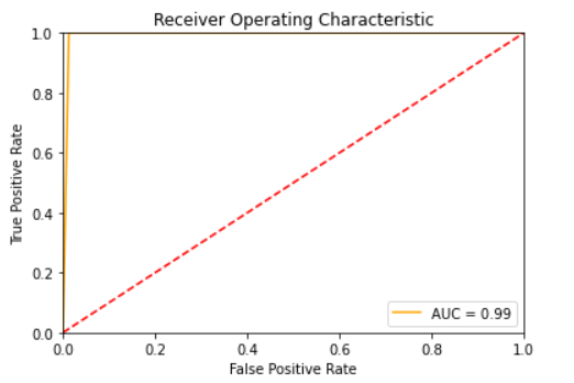
從結果可看出，不管是Accuracy或是AUC的直接為0.99，代表此模型的泛化能力 (Generalization)好。

程式碼已上傳至我的Github

參考文獻

• Hinge loss
• 淺談機器學習的效能衡量指標 (2) -- ROC/AUC 曲線

感謝您的瀏覽，我們明天見!