前言

這幾天要來講應用在「分類」問題上的機器學習模型。預計將會介紹到

• 羅吉斯迴歸( Logistic regression )
• 線性區別分析( Linear Discriminant Analysis, LDA )
• K近鄰演算法( K Nearest Neighbors, Knn )

這幾種模型以及它們在 R 上的操作。

Classification: Logistic regression

• 機器學習: 「分類」問題
• 羅吉斯迴歸 Logistic regression
  • 模型說明
  • 建立模型
  • 預測
• 模型成效判斷
  • 混淆矩陣、準確率
  • 混淆矩陣、靈敏度、特異度
  • ROC
• [補充] Regularized logistic regression

羅吉斯迴歸 Logistic regression

羅吉斯迴歸是線性回歸的延伸，線性回歸的反應變數 (Y, target/ label) 通常是連續型的數值，但羅吉斯迴歸是應用於二元類別變數上，簡單來說就是反應變數 (Y) 只有兩個種類，例如: (0,1) / (A,B)/ (是,否)/ (有,沒有)。

[註] 羅吉斯迴歸只有限制反應變數 (Y) 是二元類別變數。
解釋變數並沒有限制，解釋變數 (X) 不論是連續數值或是類別的變數都能夠建立模型。

• 模型說明

Logistic Curve :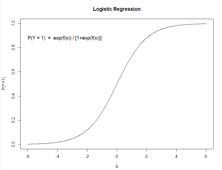

Y 為 「類別1」 的機率: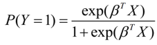

羅吉斯迴歸模型( logit link ):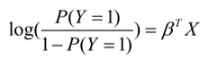

glm(y ~ x , family=, data=) 是 R 裡內建的 Generalized Linear Model( GLM ) 的廣義線性模型函數，使用方式和線性迴歸模型的 lm( )很像，Y 放”反應變數” X 放”解釋變數”。

• 建立模型

建立羅吉斯迴歸: glm(Y ~ X, family = “binomial”, data=data)
建構羅吉斯迴歸模型時，要設定 family = “binomial"，這樣才能對應到 logit link 的 Link function 上。
[補充] 其他 family type和 link function

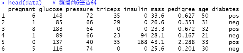
以下使用 Diabetes data 糖尿病資料做一個 Logistic regression 的小示範，這裡是示範的程式碼:
首先需要從mlbench這個package裡載入資料。
這個例子裡:

反映變數 Y: {有沒有糖尿病} (1: 沒有；2: 有)，
解釋變數 X: 有8個變數，包括 懷孕次數、血糖等等。

在建模之前一樣需要觀察一下資料的型態:

install.packages("mlbench") # Diabetes data
library(mlbench)
data("PimaIndiansDiabetes")
data<- PimaIndiansDiabetes
head(data)   # 觀看前6筆資料
summary(data)# 連續型資料:會看到 Qu.    #類別型資料:會看到不同類別的資料個數 
str(data)    # 列出資料內每個欄位的狀態

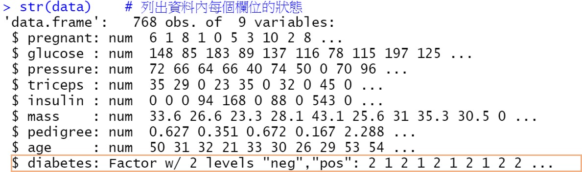
可以看到糖尿病( Diabetes )是二元的類別(Factor)變數，並且被編碼成 1("neg"), 2("pos")。

為了後續建模不希望有 Overfitting 或 Under fitting 的情況，所以我們先把資料分割為training 跟testing data，這裡舉例為 70% 、 30% 的分割，先以 training data建立模型，再以 testing data 檢驗我們的模型結果。

set.seed(1) # 固定sample()抽樣的結果
train_rows<- sample(x=1:nrow(data), size=ceiling(0.70*nrow(data) ))# 70%的data
train<- data[train_rows,] # 70%當training data
test<-  data[-train_rows,]# 30%當testing data

[注意]
⇒ glm( )函數在建羅吉斯迴歸時，需要帶入的( Y )資料為0或1的二元資料，所以要先進行資料處裡。
這裡是將 Y 直接 -1 ，變成了(0: 沒有糖尿病；1: 有糖尿病)的編碼。
如果忘了 0, 1 分別代表什麼意思，可以用contrast()函數做個確認。

#為了放入glm()，將反應變數factor從編碼"1、2" 轉成"0和1"
train$diabetes = as.numeric(train$diabetes) -1 
test$diabetes = as.numeric(test$diabetes) -1 
contrasts(data$diabetes) # neg: 0, pos: 1

接著建立羅吉斯迴歸模型( Logistic regression model )進行判斷、分類

model_glm = glm(diabetes ~ ., data = train, family = "binomial")
summary(model_glm)

> summary(model_glm)

Call:
glm(formula = diabetes ~ ., family = "binomial", data = train)

Deviance Residuals: 
    Min       1Q   Median       3Q      Max  
-2.4926  -0.7722  -0.4314   0.8022   2.7578  

Coefficients:
             Estimate Std. Error z value Pr(>|z|)    
(Intercept) -7.792026   0.838851  -9.289  < 2e-16 ***
pregnant     0.140563   0.036508   3.850 0.000118 ***
glucose      0.031374   0.004139   7.580 3.45e-14 ***
pressure    -0.015932   0.006096  -2.613 0.008965 ** 
triceps     -0.006229   0.007793  -0.799 0.424104    
insulin     -0.001126   0.001128  -0.999 0.317953    
mass         0.098980   0.018055   5.482 4.20e-08 ***
pedigree     0.812996   0.352517   2.306 0.021096 *  
age          0.011988   0.010661   1.124 0.260803    
---
Signif. codes:  0 ‘***’ 0.001 ‘**’ 0.01 ‘*’ 0.05 ‘.’ 0.1 ‘ ’ 1

(Dispersion parameter for binomial family taken to be 1)

    Null deviance: 705.70  on 537  degrees of freedom
Residual deviance: 531.35  on 529  degrees of freedom
AIC: 549.35

Number of Fisher Scoring iterations: 5

建立完羅吉斯迴歸模型，我們可以去做模型推論:
透過邏輯斯迴歸的logit link，我們可以由exp(係數beta)去解釋發生事件(Y=1, 患有糖尿病)的勝算比。
勝算比(Odds ratio)= exp(係數beta)。

舉例來說:
pregnant的coefficient 為0.14，那exp(0.14)= 1.15，表示每增加一次懷孕次數，得到糖尿病的勝算提高1.15倍。

• 預測 predict(model, type)
  除了解釋模型，我們也使用這個模型去對資料進行預測、分類。

在 R 裡建構羅吉斯迴歸時，如果要進行預測時依樣使用函式predict( )。
預設的輸出為type = "link"，輸出的值是。
當我們希望輸出一個 P(Y=1) 的機率值(介於0~1之間)時，
需要更改設定為type = "response"，這時輸出的值就會是。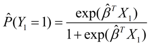

#predict(model,type,newdata)
#這裡用head()觀察predict()函數前6項輸出結果
head(predict(model_glm)) # predict()預設type="link"
head(predict(model_glm, type = "link"))# 每個樣本分別代入X的預測結果Y

## type='response'，機率P(Y=1∣X=x)
head(predict(model_glm, type='response'))
# type=link的數值經過轉換，可以變成type='response'的機率
exp(-0.4363519)/(1+exp(-0.4363519)) #以資料679為例

> head(predict(model_glm, type = "link"))
       679        129        509        471        299        270 
-0.4363519 -1.4736009 -1.8532542  0.2277766  0.2166410  0.3224093 
> head(predict(model_glm, type='response'))
      679       129       509       471       299       270 
0.3926106 0.1863959 0.1354913 0.5566992 0.5539494 0.5799113 
> exp(-0.4363519)/(1+exp(-0.4363519)) #以資料679為例
[1] 0.3926106

得到預測機率後，可以使用ifelse(result > c , 1, 0)給定一個閥值 c 去進行「分類」。
舉例來說: 如果預測機率值大於特定閥值(例如 0.5)，會將那筆資料的 Y 分類為 1，其他為0。

#得到機率後，給定一個閥值進行"分類"
result = predict(model_glm, type='response')
class_result = ifelse(result > 0.5,1,0)# 閥值c設定為0.5用來區隔不同類
head(class_result)

> head(result)
679 129 509 471 299 270 
  0   0   0   1   1   1 

如果想對新資料進行預測，使用predict( model, type, newdata) :

#自己假設一筆資料
new_data=data.frame(pregnant=0,glucose=111,pressure=62,triceps=0,
                            insulin=0,mass=22.6,pedigree=0.142,age=21)
predict(model_glm,type = "response",
        newdata = new_data)
class_result = ifelse(result > 0.5,'1: pos','0: neg')
print(class_result)

> result = predict(model_glm,type = "response",newdata = new_data)
> class_result = ifelse(result > 0.5,'1: pos','0: neg')
> print(class_result)
       1 
"0: neg" 

模型成效判斷

這裡以 training data 建立模型，再對 testing data 進行預測、分類，進而檢驗我們的模型成效。

• Cross table (Confusion Matrix) 混淆矩陣 (查看預測結果、準確率)
  我們可以輸出混淆矩陣來看看模型預測、分類 testing data 的結果和並計算準確率。

result = predict(model_glm,newdata=test,type='response')
result = ifelse(result > 0.5,1,0)
table(predicted = result, actual = test$diabetes)
#Accuracy
(143+41)/230

準確率的計算為斜對角數目(分類正確的數目)除以資料總數。

> result = predict(model_glm,newdata=test,type='response')
> result = ifelse(result > 0.5,1,0)
> table(predicted = result, actual = test$diabetes)
         actual
predicted   0   1
        0 143  31
        1  15  41
> #Accuracy
> (143+41)/230
[1] 0.8

• [進階] Confusion Matrix + Statistics 混淆矩陣、靈敏度(Sensitifity)、特異度(Specificity)

install.packages("caret")
library(caret)
confusionMatrix(data=as.factor(result),reference=as.factor(test$diabetes))

Confusion Matrix and Statistics

          Reference
Prediction   0   1
         0 143  31
         1  15  41
                                          
               Accuracy : 0.8             
                 95% CI : (0.7424, 0.8497)
    No Information Rate : 0.687           
    P-Value [Acc > NIR] : 8.356e-05       
                                          
                  Kappa : 0.5051          
                                          
 Mcnemar's Test P-Value : 0.02699         
                                          
            Sensitivity : 0.9051          
            Specificity : 0.5694          
         Pos Pred Value : 0.8218          
         Neg Pred Value : 0.7321          
             Prevalence : 0.6870          
         Detection Rate : 0.6217          
   Detection Prevalence : 0.7565          
      Balanced Accuracy : 0.7373          
                                          
       'Positive' Class : 0  

• Receiver Operating Characteristics, ROC
  除此之外，也可以畫 ROC curve 來看模型配適的好不好:

install.packages("pROC")
library("pROC")
test_prob = predict(model_glm, newdata = test, type = "response")
par(pty = "s") #指定畫布繪製成正方形的大小
test_roc = roc(test$diabetes ~ test_prob, plot = TRUE,
               print.auc = TRUE,legacy.axes=TRUE) 
#legacy.axes=TRUE 將 x軸改成 1 - Specificity

曲線下的面積稱為 AUC (Area Under Curve)，AUC面積越大越好，表示模型配適越好。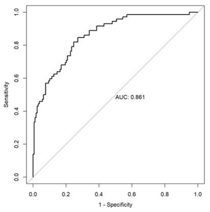

[補充]Regularized logistic regression

羅吉斯迴歸也同樣能進行正規化，和一般正規化迴歸一樣使用 glmnet() 函式，不過裡面要設定 family = "binomial" 。

glmnet( 
    family =若y是連續值，設"gaussian" ,
            若y是二元分類，設"binomial",
            若y是多元分類，設"multinomial",
     alpha = 0(Ridge) 、介於0~1介之間(Elastic-net)、1(Lasso), 
    lambda = 懲罰值 ) 

參考資料、網站、書籍

An Introduction to Statistical Learning with Applications in R. 2nd edition. Springer. James, G., Witten, D., Hastie, T., and Tibshirani, R. (2021).