Ensemble Learing 集成學習(二) Bagging, Adaboost, Logitboost

• 前言
• Bagging、Bagging Trees
• Boosting
  • Adaboost
  • Logitboost
  • Boosting 補充

前言

今天主要會去示範昨天講過的 Bagging Trees、Boosting (Adaboost, Logitboost)在 R 上的程式碼。

主要會使用 Iris Dataset 的資料，目標設為一個二元分類問題(Iris 是否為 "virginica" 這個種類)。新增了一個變數"class_virginica"作為目標(Y, Target)，若是 virginica 變數則為"1"，其餘為"0"。

# Set a two class, binary classification problem
data("iris")
df_iris=iris
df_iris$class_virginica[df_iris$Species=="virginica"]<- 1#"virginica"
df_iris$class_virginica[df_iris$Species!="virginica"]<- 0#"others"
df_iris$class_virginica<-as.factor(df_iris$class_virginica) #提醒class_virginica為二元分類類別變項
df_iris=df_iris[,-5]
head(df_iris)
# 切分資料
set.seed(123)
index.train.iris = sample(1:nrow(df_iris), size=ceiling(0.8*nrow(df_iris)))
train.iris = df_iris[index.train.iris, ]
test.iris = df_iris[-index.train.iris, ]

> head(iris[index.train.iris, ])
    Sepal.Length Sepal.Width Petal.Length Petal.Width   Species
14           4.3         3.0          1.1         0.1    setosa
50           5.0         3.3          1.4         0.2    setosa
118          7.7         3.8          6.7         2.2 virginica
43           4.4         3.2          1.3         0.2    setosa
150          5.9         3.0          5.1         1.8 virginica
148          6.5         3.0          5.2         2.0 virginica
> head(df_iris[index.train.iris, ])
    Sepal.Length Sepal.Width Petal.Length Petal.Width class_virginica
14           4.3         3.0          1.1         0.1               0
50           5.0         3.3          1.4         0.2               0
118          7.7         3.8          6.7         2.2               1
43           4.4         3.2          1.3         0.2               0
150          5.9         3.0          5.1         1.8               1
148          6.5         3.0          5.2         2.0               1

Bagging、Bagging Trees

Bagging

如果是一般的 Bagging 模型並使用平均法整合。可以直接建立多個模型後，將多個模型預測出的結果直接加總除以模型總數，得出 Bagging 模型的預測分類結果。這裡就先不做示範了。

Bagging Trees

想在 R 裡建 Bagging Trees ，可以使用套件ipred，中的bagging( )函式。

#install.packages("ipred")
library(ipred)  # Bagging Trees

# make bootstrapping reproducible
set.seed(123)
# train bagged model
bagged_m1 <- bagging(
  formula = class_virginica ~ ., # Y, Target目標變數
  data    = train.iris, # Training data訓練集資料
  coob    = TRUE # Use the OOB sample to estimate the test error
)
bagged_m1

Bagging regression trees with 25 bootstrap replications 
Call: bagging.data.frame(formula = class_virginica ~ ., data = train.iris, 
    coob = TRUE)

Out-of-bag estimate of root mean squared error:  0.2141 

內建是建立25棵樹，並輸出 Out-of-bag Root mean squared error 的結果。

當然我們也能建多個不同數目的 Bagging Trees Models 去做比較，這時只要設定好種子數(set.seed( ))，就能畫出不同 ntree 下對應的 OOB RMSE 。

set.seed(123) #種子數，固定抽樣的原則，讓人能重現模型
# 嘗試10-90 bagged trees
ntree <- seq(10,90,2)

# create empty vector to store OOB RMSE values
rmse <- vector(mode = "numeric", length = length(ntree))

#不同 ntree 數值建立出的 Bagging Trees
for (i in seq_along(ntree)) {
  # reproducibility
  set.seed(123)
  
  # perform bagged model
  model <- bagging(
    formula = class_virginica ~ .,
    data    = train.iris,
    coob    = TRUE,
    nbagg   = ntree[i]
  )  
  rmse[i] <- model$err # get OOB error
}
## plot
plot(ntree, rmse, type = 'l', lwd = 2,ylim = c(0.2, 0.23))
abline(v = 65, col = "red", lty = "dashed")

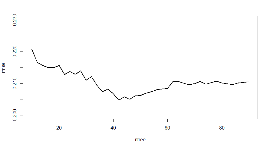
這邊我們可能會去選 65棵左右的 Trees 數目，因為在65附近可以看到 validation error 逐漸平緩。

Boosting

Boosting模型演算法如以下示意圖: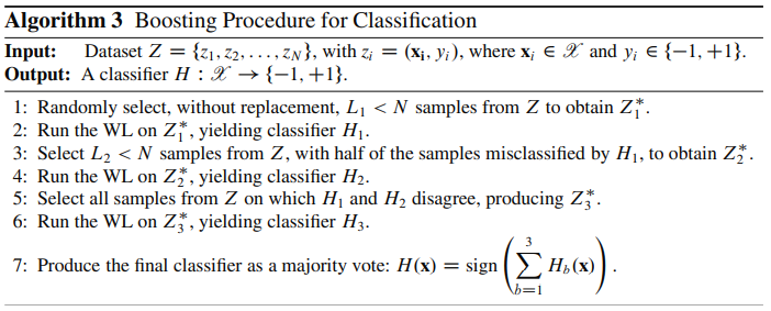

接下來會補充幾個 Boosting 延伸出的模型的程式碼。

Adaboost

Adaboost ( Adaptive Boosting 自適應增強)模型演算法的架構如以下示意圖: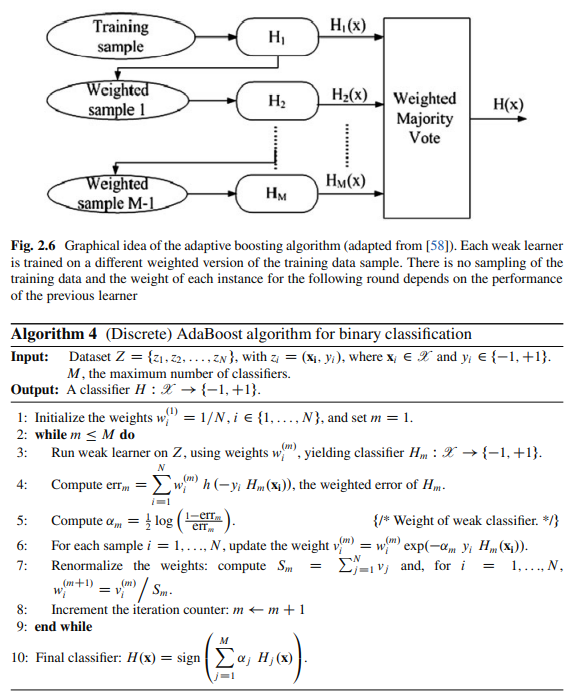

想在 R 裡建 Adaboost model，可以使用套件adabag，中的boosting( )函式。

基礎模式:

boosting (formula = Y~X,
 	boos      = TRUE, #(默認) 權重使用迭代時的權重/ FALSE 觀測值使用相同的權重。,
    mfinal    = ntree, # Number of Trees (迭代的最大次數)，預設100。,
	Maxdepth  = mdp, # Max Tree Depth,
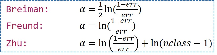
    coeflearn = “Breiman” # (?, weight updating coefficient)權重計算方法。“Breiman”（默認）, "Freund", "Zhu"
... ) 

adabag 套件詳細說明連結。

範例:

#install.packages("adabag")
library(adabag)
library(rpart.plot)

# 用boosting（）建立adaboost
ad.iris=boosting(class_virginica~.,data=df_iris,mfinal=60) # mfinal設定迭代的次數，預設100

summary(ad.iris)
ad.iris$trees # 內部的決策樹長相
ad.iris$weights
ad.iris$importance

barplot(sort(ad.iris$importance))             # 畫出變數重要性圖
importanceplot(ad.iris)                       # 畫出變數重要性圖(用library(rpart.plot))

# predict()
iris.ad.pred <- predict(ad.iris, test.iris)$class #記得加$class
table(observed=test.iris$class_virginica , predicted = iris.ad.pred) # Confusion matrix
mean(test.iris$class_virginica==iris.ad.pred )                       # Accuracy=對角線占比

# 在使用library(adabag)時，package內含的Confusion matrix、Accuracy的函數:
predict(ad.iris, test.iris)$confusion             # Confusion matrix
1 - predict(ad.iris, test.iris)$error             # Accuracy=1-error%


# mfinal設定迭代的次數，預設100
error.lv<-errorevol(ad.iris,train.iris)
# 誤差vs迭代數
plot(error.lv$error,type="l",main="AdaBoost error vs number of trees",xlab ='Iterations' , xlim=c(0,15), ylim=c(0,0.08)) 

# Comparing error evolution in training and testing set
error.lv.tr<-errorevol(ad.iris,train.iris)
error.lv.te<-errorevol(ad.iris,test.iris)
plot.errorevol(error.lv.te, error.lv.tr)
plot.errorevol(error.lv.te, error.lv.tr, xlim=c(0,15), ylim=c(0,0.08))

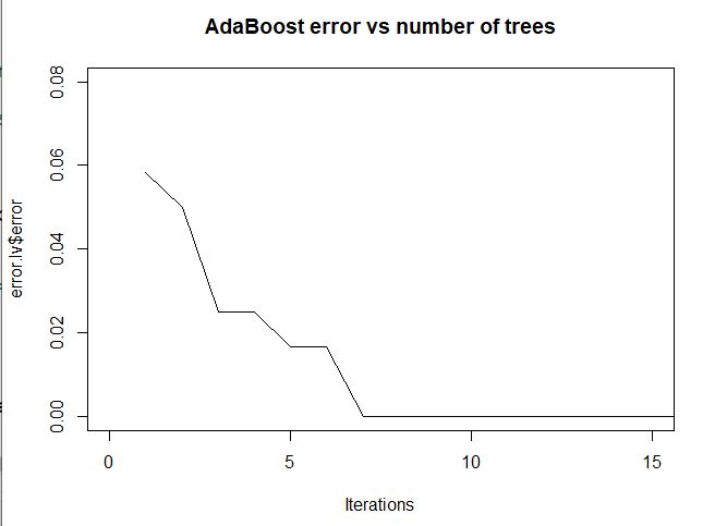
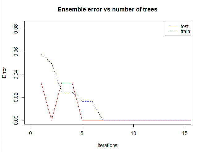
從圖中可以看出來，由於資料本身不複雜，其實迭帶7次左右就有不錯的結果。

一樣我們可以用變數重要性圖去觀察什麼變數是影響分類的重要變數: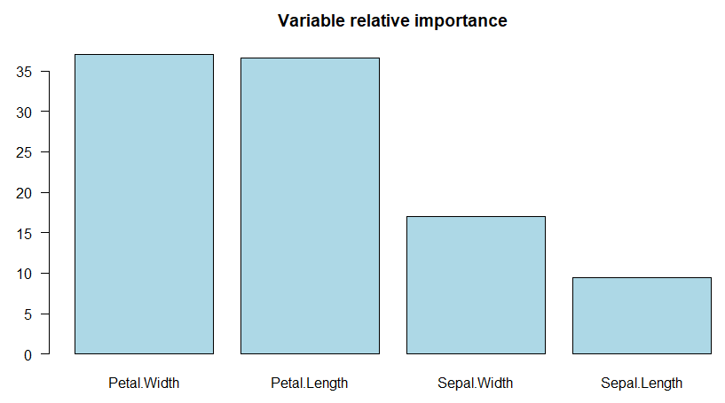

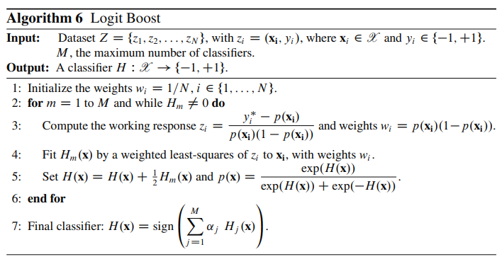
Logitboost

If one considers AdaBoost as a generalized additive model and then applies the cost function of logistic regression, one can derive the LogitBoost algorithm.
LogitBoost, From Wikipedia

Logitboost 的模型演算法架構如以下圖:

想在 R 裡建 Logitboost ，可以使用套件caTools，中的LogitBoost(xtrain, ytrain, nIter=i)函式。

基礎模式:

LogitBoost( xlearn    = X  ,#X Data,
    	     ylearn    = Y ,#Y Label,
    	     nIter     = i ,#the number of iterations
)
           ``` 
[caTool]( https://cran.r-project.org/web/packages/caTools/caTools.pdf) 套件詳細說明連結。

範例:
``` R
#install.packages("caTools")
library(caTools)
set.seed(123)
names(iris)
index.train.iris = sample(1:nrow(iris), size=ceiling(0.8*nrow(iris)))
train.iris = iris[index.train.iris, ]
test.iris = iris[-index.train.iris, ]

xtrain = train.iris[, -5] #only x
ytrain = train.iris[, 5]  #only y
xtest = test.iris[, -5]   #only x
ytest = test.iris[, 5]    #only y

logBoost = LogitBoost(xtrain, ytrain, nIter=50)
iris.logBoost.pred = predict(logBoost, xtest)  
table(observed=test.iris$class_virginica , predicted = iris.logBoost.pred) # Confusion matrix
mean(test.iris$class_virginica==iris.logBoost.pred )                       # Accuracy=對角線占比

Boosting 補充

• Gradient Boosting Machine，都可以使用套件Caret，中的train(method = “gbm”)函式去建立模型。

• XGboost，可以使用套件xgboost，中的xgb.train()函式去建立模型。

[補充]
當我們遇到了一個二元分類問題，除了建立模型後去觀察準確率，也可以去試著畫 ROC Plot ，看看模型分類氣的好壞。 ROC Plot 可以使用 R 裡的pROC套件中的roc( )函式。

參考資料、網站

Ensemble Machine Learning Methods and Applications. Zhang, Cha., and Yunqian. Ma. Edited by Cha Zhang, Yunqian Ma. Boston, MA: Springer US. (2012).

R筆記 – (16) Ensemble Learning(集成學習)(@skydome20)
https://rpubs.com/skydome20/R-Note16-Ensemble_Learning
AFIT Data Science Lab R Programming Guide Regression Trees
https://afit-r.github.io/regression_trees