決策樹(剪枝)、隨機森林(超參數選擇)、重要變數 [PYTHON 補充 ]

• 前言、使用資料
• CART Tree模型、複雜度參數Cp選擇
• 隨機森林模型 n_estimators 、 max_feature選擇

前言、使用資料

昨天補充了建立多個模型，以及如何輸出各個模型的模型評估指標，還有他們是如何計算得出那些數值。
今天要補充建立其中的決策樹和隨機森林模型時，如何調整模型的超參數。

• 調整模型超參數:

1. 決策樹的參數調整是去選擇用來剪枝的複雜度Cp(complexity parameter)。
2. 隨機森林的參數調整包含選擇n_estimators(森林裡要建幾棵樹) 和 max_feature(每棵樹要抽多少解釋變數去建立)等等。

以下範例使用 Breast Cancer Dataset，目標變數Target 分為兩類'malignant'惡性, 'benign'良性腫瘤。資料集內含有30個連續型的解釋變數，共有569筆資料。
資料來源:Breast Cancer Wisconsin (Diagnostic) Data Set。
載入套件:

import pandas as pd
import numpy as np
import matplotlib.pyplot as plt
import seaborn as sns
import statsmodels as sm
## Common imports
import sys
import sklearn # scikit-learn
import os
import scipy
## plot
import matplotlib as mpl
import matplotlib.pyplot as plt

## 分割資料
from sklearn import datasets
from sklearn.model_selection import train_test_split

## modelbuilding 模型套件
from sklearn.tree import DecisionTreeClassifier
from sklearn.ensemble import RandomForestClassifier

載入資料:

from sklearn.datasets import load_breast_cancer
breast_cancer=datasets.load_breast_cancer()
x, y = datasets.load_breast_cancer(return_X_y=True)
x_train,x_test,y_train,y_test=train_test_split(x,y,test_size=0.2)

###  CART Tree模型、複雜度參數Cp選擇
- 基礎的決策樹模型以及常用的調整說明:
``` PYTHON
from sklearn import tree
DecisionTreeClassifier(
    criterion='gini', # 樹分割的criterion有:“gini”, “entropy”, “log_loss”
    max_depth=None, #決策樹的深度
    min_samples_split=2, #內部節點至少需要多少資料數目，才去進行劃分
    min_samples_leaf=1, #每個最末節點(葉子)至少要有多少資料數目(samples)。
    max_features=None,  #最多使用多少變數去建立樹。
    random_state=None,  # Controls the randomness of the estimator. 
    max_leaf_nodes=None, #最末節點(葉子)數目
    min_impurity_decrease=0.0, #分類類別至少的純淨度。
    ccp_alpha=0.0  #剪枝用的複雜參數，Complexity parameter (used for  Minimal Cost-Complexity Pruning)
    )

若是想要建立迴歸樹，可以使用套件 from sklearn.tree import DecisionTreeRegressor 中的函式DecisionTreeRegressor()。

挑選複雜度參數Cp

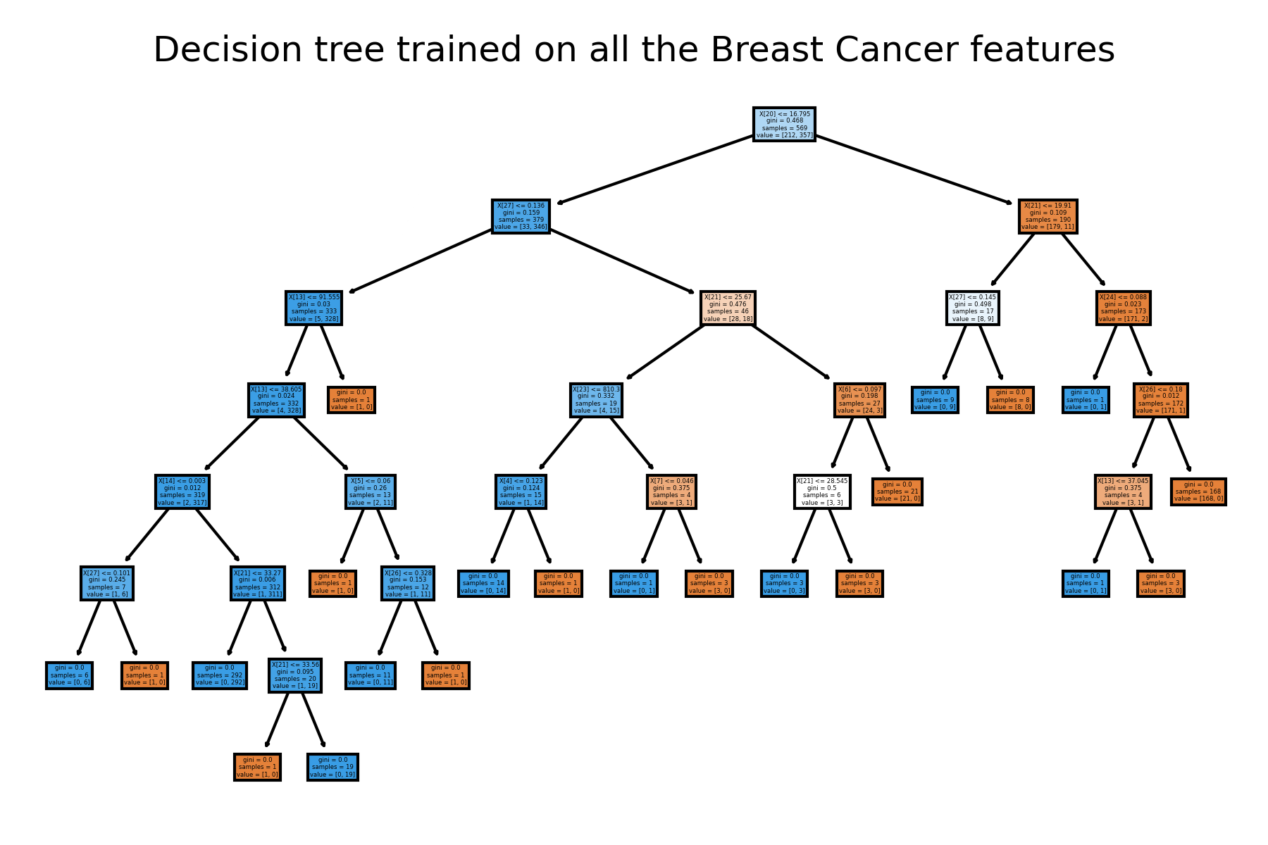
原始不做篩選的樹長這樣:

from sklearn.tree import plot_tree #圖
# 普通不設限制的決策樹
clf = DecisionTreeClassifier()
clf = clf.fit(x, y)
plt.figure()
tree.plot_tree(clf, filled=True) #filled=True套色
plt.title("Decision tree trained on all the Breast Cancer features")
plt.show()

我們可以畫出不同Cp下的模型對應到的 train, test data error:

clf = DecisionTreeClassifier(random_state=0)
path = clf.cost_complexity_pruning_path(x_train, y_train)
ccp_alphas, impurities = path.ccp_alphas, path.impurities

clfs = []
for ccp_alpha in ccp_alphas:
    clf = DecisionTreeClassifier(random_state=0, ccp_alpha=ccp_alpha)
    clf.fit(x_train, y_train)
    clfs.append(clf)
print(
    "Number of nodes in the last tree is: {} with ccp_alpha: {}".format(
        clfs[-1].tree_.node_count, ccp_alphas[-1]
    )
)


train_scores = [clf.score(x_train, y_train) for clf in clfs]
test_scores = [clf.score(x_test, y_test) for clf in clfs]

fig, ax = plt.subplots()
plt.xlim(-0.01,0.04)
plt.ylim(0.8,1.05)
ax.set_xlabel("alpha(Cp)")
ax.set_ylabel("accuracy")
ax.set_title("Accuracy vs alpha for training and testing sets")
ax.plot(ccp_alphas, train_scores, marker="o", label="train", drawstyle="steps-post")
ax.plot(ccp_alphas, test_scores, marker="o", label="test", drawstyle="steps-post")
ax.legend()

plt.show()

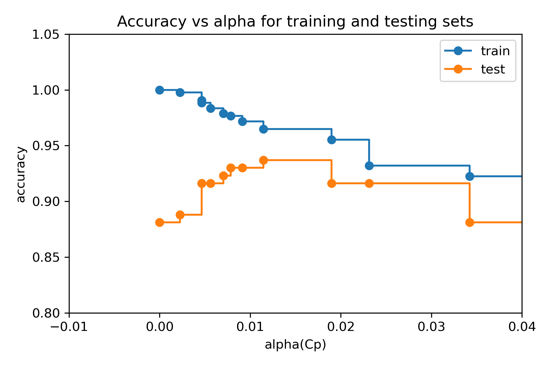
這裡可能會去選擇Cp (alpha) = 0.01 作為參數。
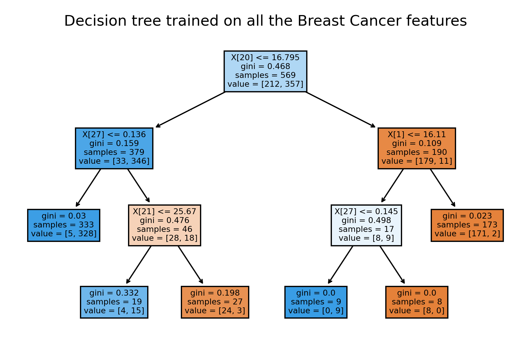
在只去挑選Cp的情況下，最終決策樹模型為:

DecisionTreeClassifier(random_state=0, ccp_alpha=0.01).fit(x_train, y_train)

clf = DecisionTreeClassifier(ccp_alpha=0.01)
clf = clf.fit(x_train, y_train)
plt.figure()
tree.plot_tree(clf, filled=True) #filled=True套色
plt.title("Decision tree trained on all the Breast Cancer features")
plt.show()

想測試其他設限時，也可以自記寫迴圈測試比較不同數值限制下的模型表現。

隨機森林模型 ntree、mtry 選擇

• 基礎的隨機森林模型:

RandomForestClassifier(n_estimators=100, # ntrees
                       criterion='gini', 
                       max_depth=None, 
                       min_samples_split=2, 
                       min_samples_leaf=1,
                       max_features='sqrt', #mtry
                       max_leaf_nodes=None, 
                       min_impurity_decrease=0.0, 
                       bootstrap=True, #bootstrap samples are used when building trees
                       oob_score=False, #ut-of-bag samples to estimate the generalization score
                       random_state=None,
                       ccp_alpha=0.0)

挑選 n_estimators 、 max_feature

在建立隨機森林模型時我們通常會去調整 n_estimators(R 裡的 ntree)和max_feature(R 裡的 mtry)。
在這裡我們可以畫出不同max_feature的模型，在對應建立不同樹木的樹時的OOB Rate。

from collections import OrderedDict

RANDOM_STATE = 123
# NOTE: Setting the `warm_start` construction parameter to `True` disables
# support for parallelized ensembles but is necessary for tracking the OOB
# error trajectory during training.


ensemble_clfs = [
    
    (
        "RandomForestClassifier, max_features=5",
        RandomForestClassifier(
            warm_start=True,
            oob_score=True,
            max_features=5,
            random_state=RANDOM_STATE,
        ),
    ),
    (
        "RandomForestClassifier, max_features=15",
        RandomForestClassifier(
            warm_start=True,
            max_features=15,
            oob_score=True,
            random_state=RANDOM_STATE,
        ),
    ),
    (
        "RandomForestClassifier, max_features=None",
        RandomForestClassifier(
            warm_start=True,
            max_features=None,
            oob_score=True,
            random_state=RANDOM_STATE,
        ),
    ),
]


# Map a classifier name to a list of (<n_estimators>, <error rate>) pairs.
error_rate = OrderedDict((label, []) for label, _ in ensemble_clfs)

# Range of `n_estimators` values to explore.
min_estimators = 30
max_estimators = 500

for label, clf in ensemble_clfs:
    for i in range(min_estimators, max_estimators + 1, 5):
        clf.set_params(n_estimators=i)
        clf.fit(x_train, y_train)

        # Record the OOB error for each `n_estimators=i` setting.
        oob_error = 1 - clf.oob_score_
        error_rate[label].append((i, oob_error))

# Generate the "OOB error rate" vs. "n_estimators" plot.
for label, clf_err in error_rate.items():
    xs, ys = zip(*clf_err)
    plt.plot(xs, ys, label=label)

plt.xlim(min_estimators, max_estimators)
plt.ylim(0, 0.08)
plt.xlabel("n_estimators")
plt.ylabel("OOB error rate")
plt.legend(loc="upper right")
plt.show()

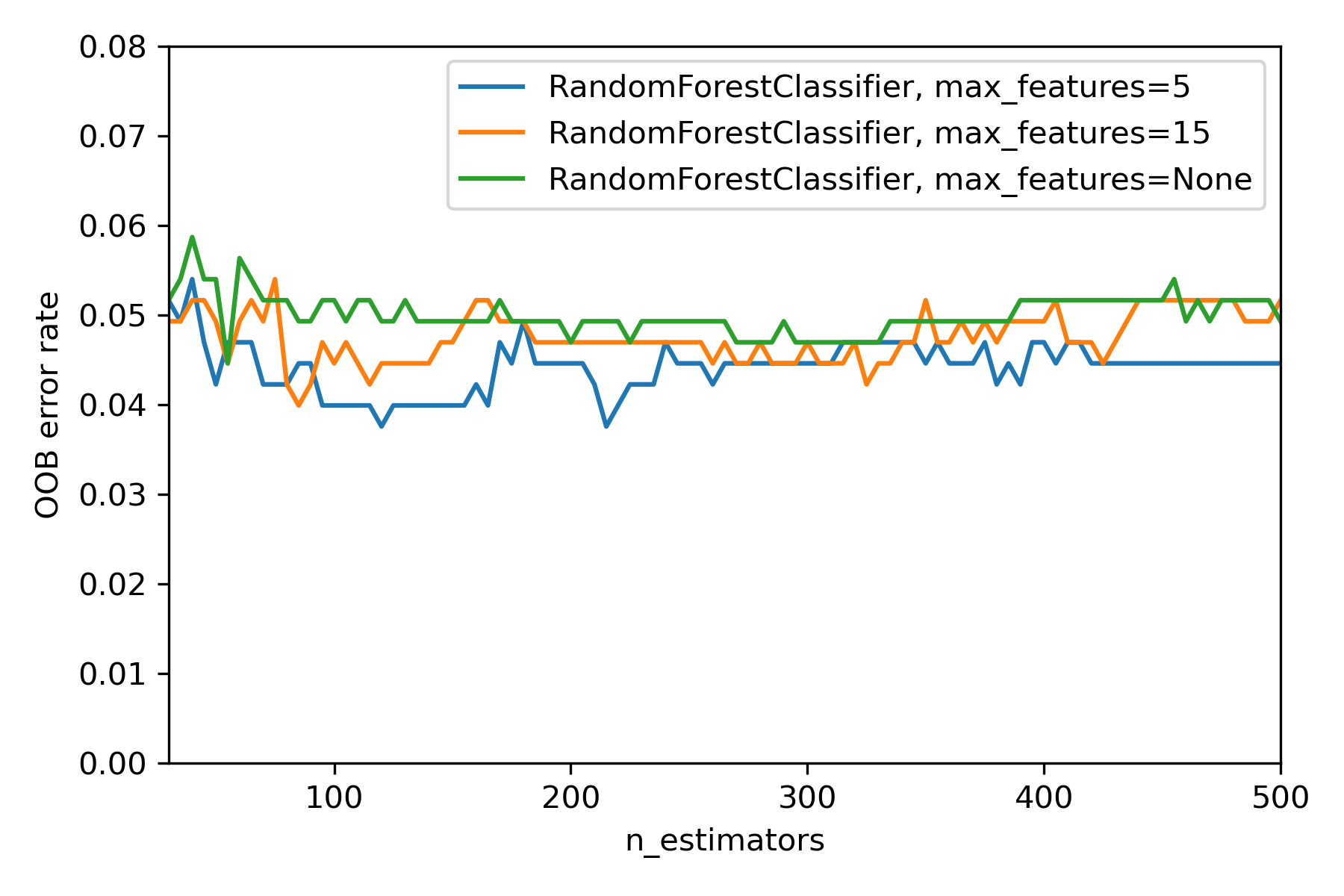
這裡可能會去選擇 n_estimators=300 , max_feature=5作為參數。
在只去挑選 n_estimators 和 max_feature 的情況下，最終隨機森林模型為:

RandomForestClassifier(n_estimators=300,max_features=5,random_state=0)

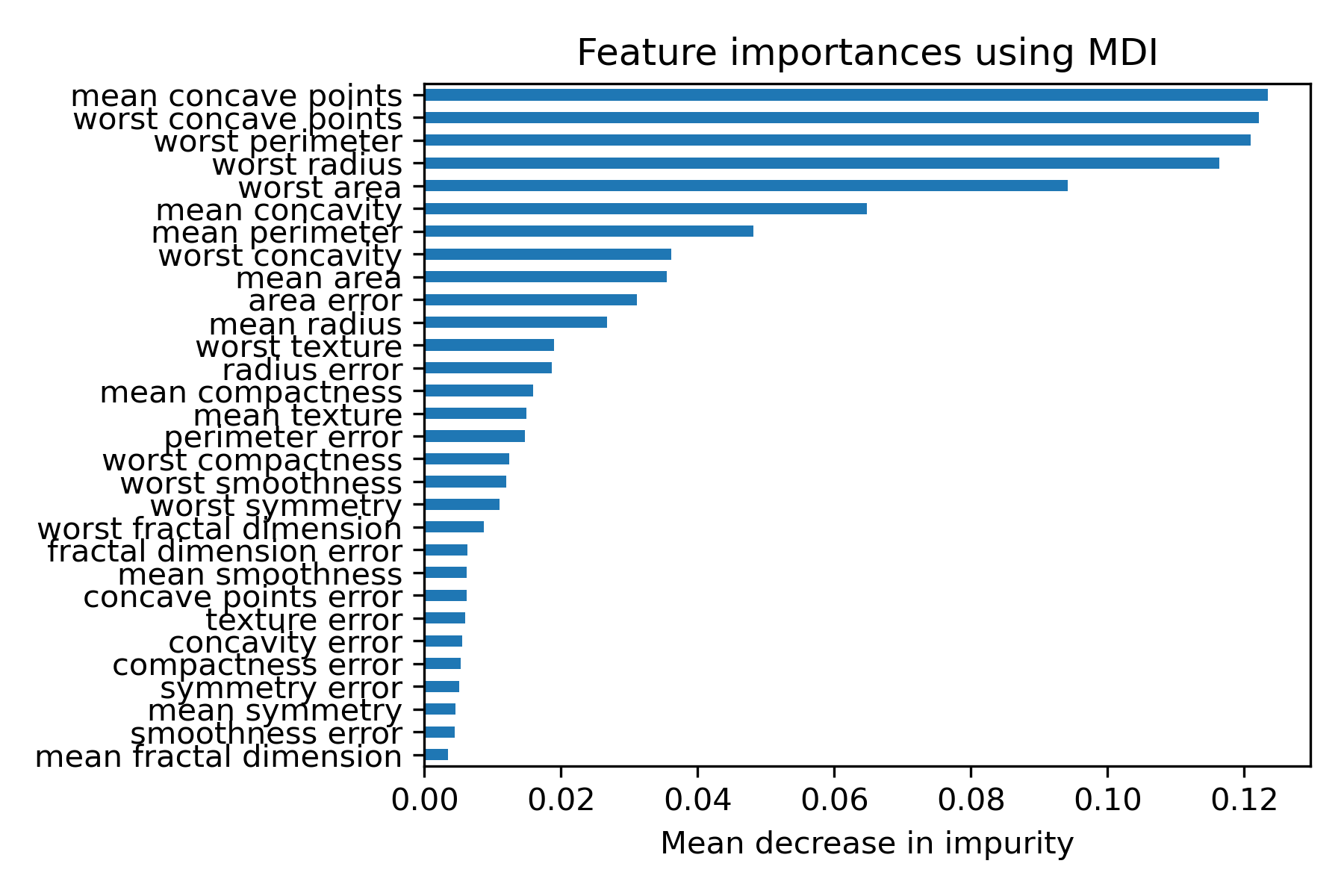
建完模型後，可以藉由feature_importances_Mean Decrease in Impurity(MDI) 幫我們去了解各解釋變數對模型的影響力(變數重要性)。

import numpy as np
feature_names=datasets.load_breast_cancer(as_frame=True).feature_names
forest = RandomForestClassifier(n_estimators=300,max_features=5,random_state=0)
forest.fit(x_train, y_train)

importances = forest.feature_importances_
forest_importances = pd.Series(importances,index=feature_names).sort_values(ascending=True)

fig, ax = plt.subplots()
forest_importances.plot.barh( ax=ax)
ax.set_title("Feature importances using MDI")
ax.set_xlabel("Mean decrease in impurity")
save_fig("rftune_varplt")
fig.tight_layout()

參考資料、網站

sklearn.tree.DecisionTreeClassifier
https://scikit-learn.org/stable/modules/generated/sklearn.tree.DecisionTreeClassifier.html#sklearn.tree.DecisionTreeClassifier

Post pruning decision trees with cost complexity pruning
https://scikit-learn.org/stable/auto_examples/tree/plot_cost_complexity_pruning.html#sphx-glr-auto-examples-tree-plot-cost-complexity-pruning-py

OOB Errors for Random Forests
https://scikit-learn.org/stable/auto_examples/ensemble/plot_ensemble_oob.html#sphx-glr-auto-examples-ensemble-plot-ensemble-oob-py

Feature importances with a forest of trees
https://scikit-learn.org/stable/auto_examples/ensemble/plot_forest_importances.html#sphx-glr-auto-examples-ensemble-plot-forest-importances-py